ESCI 407/507: Forest Ecology

Spring 2024

Last updated: 4/19/2024:

We will initially meet in ES322 for lab this week

Bring a Thumbdrive (USB drive) to lab. You will need it to transfer data.

SNOWPACK DATA INCLUDED BELOW (updated 4/17/2024)!!!

Lab #3: Climatic, Edaphic and Biological Controls on Tree Growth
PART III: Ring Width Measurement and Data Analysis

A. LAB WORK:

1) Preliminary Examination: Each of the increment cores that we collected last week has been sanded to make the rings easier to see. Take a look at your core under a dissecting microscope. The first full ring on each core will be for the previous (2023) growing season. It is still too early in the year for trees to show any growth for the upcoming (2024) growing season. As you know from reading Fritts (1971; you should have read this last week. fritts_1971.pdf ), the patterns that we recognize as growth rings are formed from the alternating bands of light colored spring wood (also referred to as earlywood) and darker bands of summer wood (also known as latewood). Here is an example:

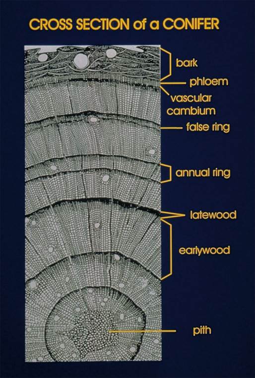
(source: http://www.ngdc.noaa.gov/paleo/slides/slideset/18/index.html)

During the spring and early summer when nutrients and water are abundant, the tree is growing rapidly and the wood has a lower density and the individual cell walls that make up the wood are relatively thin. In the late summer, the growth rate declines and the wood has a higher density and the individual cell walls are much thicker. Within a single growing season, conditions change slowly so the transition (boundary) from spring wood to summer wood is rather fuzzy. In contrast, the boundary between the late summer wood of one year and the spring wood of the next growing season is very sharp. Take a careful look at your core and make certain that you can see this difference. With the bark-end of the core on your left, the left-hand side of each dark band should be rather sharp and the right-hand side of each dark band should be rather fuzzy. If your core broke before you got it glued down last week, carefully examine the entire length of the core and make certain that you did not invert any of the pieces as you were gluing them down.

2) Counting and Labeling Your Cores: Before we begin measuring individual ring widths, we will need to CAREFULLY count the rings on your core. Start at the bark and count towards the center of the tree. Use a pencil to make a mark on the mounting stick to label the ring for the beginning of each decade (2020, 2010, 2000, 1990, 1980, 1970...). These marks will be useful reference points for you when you start measuring ring widths. Take your time with this! Mis-counting or missing a ring at this point will seriously compromise our analysis. For this analysis, we will only be using data from 1994 to the present from each core. Just for fun, it would be nice to know the total number of rings in each core so go ahead and count all the rings. Be very very very careful to make sure that your count of the rings from 1994 to the present is accurate!

3) Cross-dating: Based on an examination of several cores from Mt. Baker, I found that the late 1999 usually shows up as a year of reduced growth for many, but not all, trees. Many of you may recall that this is the summer following the record setting snowfall at Mt. Baker. Although a large snowpack means more water, it also means that the snow doesn’t melt until well into the summer. This results in a shortened growing season and an narrow ring. Not all trees will show this. Nevertheless, take a look at your cores for evidence of this. This may provide a reference point for checking your counts. I am not certain how reliable this will be.

Record the total number of rings on your core and, if possible, estimate the origin date for the tree. In many (most?) cases, you will not be able to establish an exact origin date.

4) Measuring Ring Width:. In past years, we simply used dissecting microscope and a millimeter ruler to measure the width of the last ten annual rings in your core. This year, we will be using a far more accurate tree ring measuring device for this. This instrument will enable us to measure ring widths to the nearest 0.001 mm. Through Dr. Andy Bunn, a faculty member in ESCI, we have access to two of these tree ring measuring devices. I will do a demo of the device for the class and then I will work with groups of two students at a time to assist you with taking these measurements. We will begin taking measurements going back to the year 1994. Ideally, we would get a width measurement for every single ring in the core. This is quite tedious and past experience has indicated that people make lots of errors when we have attempted to do this (especially when we used a millimeter rule to take the measurements!). On a long core, it is easy to get mixed up and skip a ring or measure the same ring twice. Measure the width of each ring carefully!

Brief Instructions for Dr. Bunn’s Tree Ring Measurement Device: There are two measurement devices in his lab. Both include a computer, a microscope, a mechanical stage for the microscope and associated measurement box.

-Start the computer, turn on measurement box and microscope light

-Initialize the software: Start-Programs-Tellervo. You may need to configure the software. The steps are:

“Welcome to Tellervo”, hit next

Choose Tellervo-lite, next

Yes, I’d like to configure a measuring platform, next

On the Measuring platform configuration window, use these settings:

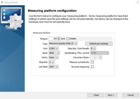
On the Test your measuring platform window, hit the rest button to zero the measurement, then turn the crank and hit the Print button. You should see a measurement get recorded. All is good.

In the Setup complete window, hit finish and you are ready to go.

-In the main Tellervo window, hit the large green sign to start a new series Series-New. Enter ID# (your initials and a number, e.g. DW1; note that this ID# should be written somewhere on the mounting stick for your core) and the start year (this is the year of the ring closest to the bark. Set MODE to “Fix Last Year Of Growth” (FLYOG). This means that we will begin with the most recent year and work backwards. Click on the “Measuring Start” button. You will be prompted to enter an initial starting value.

-In scope, place the bark-end of your core on the left. Line up the indicator line with the end of the most recent ring (interface between the wood and the bark), hit the zero button on the tree ring measuring box or the reset button on the small mouse-like thing attached to the microscope stage. On the measurement box, you will note that the value there is now reset to zero.

-Hit the “measure” icon on the top ribbon bar on the Tellervo window

-Turn crank on the stage to get to end of first ring, press the “Print” button (Note that these buttons require a rather firm push to register; there should be a beep if you pushed it properly). You will hear a beep and the ring width for the first ring will be recorded in the Tellervo window.

The measurements are to the nearest 1/1000^th of a millimeter. Note that we can’t enter a starting year so each measurement is simply given a relative year. We know that the first ring on your core (adjacent to the bark) is for the 2023 growing season. This first ring will be assigned a “year” of 1001, the next 1002 and so on. We will assign the correct years later as we work with the data in Excel.

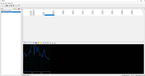
-Continue for subsequent rings. After every ten years you will (may??) hear a slightly different sounding beep (a sort of “booop”). This enables you to check to make sure you have not missed a ring. I want you to measure the first 30 rings. This will take us back to 1993. After measuring 30 rings, the Tellervo window will look like this:

-NOTE: if you have any breaks (gaps) in your core, you will need to CAREFULLY move the core (just the core, not the stage) to get past the gap. By doing so, your measurement will just include the ring, not the gap. Yes, this introduces some (maybe quite a bit) of error in the measurement of this ring but this is unavoidable.

-When you are done, go to File Save as and save this file to your USB drive using the core ID name you selected (probably your initials and a number). Save it as a .CSV file.

-Then hit the “Stop Measuring” button in the upper left of the Tellervo window. You will be asked if you want to delete the series and you should say yes. This clears the display for the next person.

-That’s it you are done here. Head down to AH05 to begin your analysis.

-File will be saved in a weird format. Convert to a more useful format using program called FMT.exe located in C:\users\wallin\esci407\ Follow onscreen instruction for this program. Read the screen prompts carefully. For the most part, you will take the default selection to almost every program prompt (by pressing the return (enter) on your keyboard). There are three prompts that will require an input:

Down in AH05, open your CSV file in Excel. You should open it as a comma delimited file. It will look something like this:

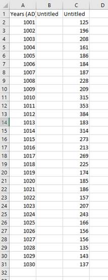
Two things here:

1. You will note that your numbers have been rounded off to 3 digits. For my first value of “125” this really means 1.25 mm. This is fine

2. Note that year “1001” is really the year 2023 and year “1030” is really 1994. In column B you can add these years.

After adding the correct years, you can then go to Data-Sort and sort your data by your new “Year” field (or in my case, the “Untitled” field). This will result in:

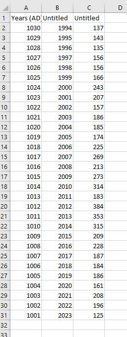
You are now ready to proceed with the analysis.

NOTE: If for any reason, the use of the new tree ring measuring device does not work, we will revert to using the millimeter rules to measure the last 10 rings on the core.

B. ANALYSIS: You now have the ring width data for your tree save as an Excel but you need to clean it up a bit. Be sure to include the ID# for your core. You can delete the first column with the 1001, 1002, etc. You want the first column to contain the year, starting with the year of your OLDEST ring. Your ring width measurements should be in the second column. We will analyze our data using linear regression analysis. Prior to lab, you should review your statistics book to refresh your memory on the use of this technique. Virtually any statistics package could be used for conducting this analysis. I will include instructions for doing this analysis using Excel. If you are more comfortable with another statistics package, feel free to use it.

1) Ring-width standardization: We need to begin by converting our raw ring-width data into a standardized ring-width index. This corrects for variation in tree size and age-related variation in growth rate. To do this,

a) Go to the Data tab, then, Data Analysis and select Regression from the list of statistical tests. Click on OK.

b) For the "Y input range," enter the ring-width values by pointing to the appropriate column (column B if you entered the data as directed), starting with the oldest ring-width measurement and dragging down to the bottom of your data (to the ring-width measurement for 2023). For the "X input range," enter the years by pointing to the appropriate column (column A if you entered the data as directed) and dragging down to the bottom of your data (to the year 2023).

c) Click on the box for Residuals and then click on OK. At this point, Excel will conduct a least-squares regression analysis with ring-width as the dependent variable and year as the independent variable. You will now be looking at another page in the notebook that holds the results of your analysis. It should look much like this:

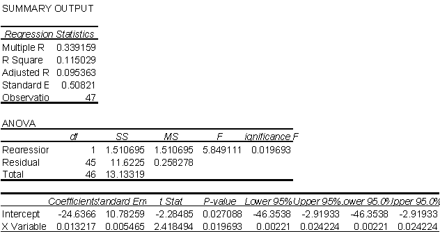
The most important values in the table above are the "Adjusted R-square" value and the "Significance of F." The latter value is the result of testing the null hypothesis that the slope of the regression line is zero. The R-square value tells you how much of the variance in ring-width is explained by the independent variable (year or tree age). The "Intercept" and "X-variable" coefficients are the "a" and "b" in the equation for our regression line, Y = a + bX.

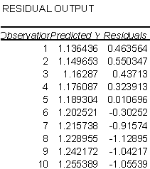
Each observation in this "residual output" section represents one year in your data set. Observation #1 is the first year in your data set. The key values here are the Predicted Y. If you plug the year into the equation above, you will get the Predicted Y.

d) To calculate standardized ring-width, make a note of the Sheet number and address of the cell that contains the first predicted Y value. Now go back to Sheet 1 in your notebook. Go to column C. In the cell adjacent to your first measured ring-width. Enter "=Sheet#!cell address" where # is the number of the sheet with the predicted Ys and cell address is the address of the first predicted Y. If you did this correctly, you have just created a link between pages in your notebook (You’ve just learned yet another Excel trick!). OK, now copy this cell to the rest of the cells in this column. I know, I know, you could have also just copied and pasted the data directly from the results sheet to this position on Sheet 1 but this would not have been nearly as cool. Finally, to get your standardized ring-width index, go to column D and enter "=B?/C?" where ? is the appropriate row number. Copy this formula to every cell in column D. Column D is our standardized ring-width index.

2) What the heck did we just do? OK, so you can follow a cookbook but do you really understand what we just did? Why did we do it? Let's back up for a minute.

a) Calculate the average of columns B,C &D: You will note that the average of columns B and C are identical and the mean of column D is very close to one (give or take some round-off error). Values in column D that are above one represent years when the tree was growing a bit faster than predicted and values below one represent year in which the tree was growing a bit more slowly than predicted. This variation may be related to climate. The standardized ring-width index removes any age-related variation in ring width from our data. With this age-related "noise" removed from our data set we can more easily look for the effect of climate on tree growth. RWI also “corrects” for differences in site quality and overall tree vigor. What does this mean? Just by chance, some trees happen to be growing in particularly good sites with abundant water and nutrients and others are growing on poor sites. On average, the trees on good sites will have wider rings than the trees on poor sites. For the purposes of this analysis, we aren’t really interested in this. We want to focus on the year-to-year variation. The use of RWI rather than raw ring widths helps us do this. Important Note: If the mean of column D is not very, very close to 1.0 (somewhere between 0.999 and 1.001) then you made a mistake and you should go back and check your work!

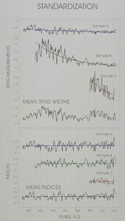
b) Plot Ring-width and Ring-width Index vs. Year: These plots might help you visualize your data.

The following figure (from another paper by Fritts) illustrates the difference between raw tree ring data and ring width index

(source: http://www.ncdc.noaa.gov/paleo/slides/slideset/18/18_366_slide.html)

3) PRELIMINARY Climate Analysis: I have created an updated version of the Climate data that you downloaded during the first lab. Click here to get a copy of this updated file. (file updated for 2013). Recall that you downloaded data for Precipitation, Minimum Temperature, Mean Temperature, Maximum Temperature and Precipitation. I have also added a few other variables including Vapor Pressure Deficit (VPD and Dew point. and Dew Point. I have also done a few additional calculations using Average Temperature and Dew Point Temperature to generate data sets for Relative Humidity (%), Saturation Vapor Pressure (mb), Actual Vapor Pressure (mb) and Vapor Pressure Deficit (mb). Of these, Vapor Pressure Deficit (VPD) is a particularly important variable that indicates moisture stress for plants. Here is a link to this file:

I will add a link to the 2024 climate data here: 2024Climate_Data.xlsx NOTE: Correction made to this file on 4/17; The version that was posted earlier had an error in the water year PPT data. The earlier version had the values off by one year. This means that, for example, the 2003 WY value was calculated using Oct-Dec of 2003 and Jan-Sept of 2004. This is incorrect. The 2003 WY should be calculated using Oct-Dec 2002 and Jan-Sept of 2003. I’ve fixed this in the attached file. Since you are using the 3 yr running mean of all of your climate variables, this should not make a big difference so don’t bother to redo anything. But if you are just starting, use this updated/corrected version of the data.

Note that I have I have calculated the following:

- Mean Temperature during June through September for each year (1895-present)

- Mean minimum temperature during June through September for each year (1895-present)

- Mean maximum temperature during June through September for each year (1895-present)

- Total precipitation for the "Water Year" of October through September for each year (1896-present). Note: You will not be able to calculate this value for 1895 since you would need precipitation data for October of 1894 through September of 1895.

- Mean Minimum Vapor Pressure Deficit during June through September of each year (1895-present)

Mean Maximum Vapor Pressure Deficit during June through September of each year (1895-present)

Mean Dewpoint Temperature during June through September of each year (1895-present)

On the “climsum” worksheet in this excel file, you will find :

1. Year to column A,

2. May 1 snowpack depth (see link below for “snowbaker.xls” dataset, then go to the “Data Summary” worksheet) to column B,

3. mean June-September temperature to column C,

4. mean minimum June-Sept temperature to column D,

5. mean maximum June-Sept temperature to column E and

6. total “water year” PPT for October-September to column F.

7. mean minimum VPD for June-Sept to column G

8. mean maximum VPD for June-Sept to column H

9. mean dewpoint temperature for June-Sept to column I

10. Now add the Ring-width Index for YOUR TREE to column J.

a) Regressions: Run eight different regression analyses using Ring-width Index as the response variable (Y Input Range) in all eight. Use one of the eight climate variables (May 1 snowpack, June-September mean temperature, min temp, max temp and Total PPT for October-September) as predictor variables in each regression analysis. Is there a statistically significant relationship? Which climate variable is the strongest predictor of ring-width index (i.e., which has the highest Adjusted R-square)?

b) Plots: A number of plots might be useful:

Year vs. Ring-width index, and year vs. each of the eight climate variables (a total of nine figures)

Each of the eight Climate variables vs. Ring-width Index (eight more figures).

You do not need to turn in any of these figures!

4) Final Analysis: The work described above is intended to give you a feel for the sort of analysis that is possible with these data. For your lab report, I would like you to draw upon ALL of the tree data we collected. To do this, you will need to provide Jessica and Kara with a CLEAN Excel file containing Tree ID#, species code, Diameter at Core Height, total tree age (estimate this if you missed the center of tree), whether the tree was isolated or not and if not, was it a canopy dominant tree or a sub-dominant tree, distance to the tree's two nearest neighbors and the diameters of each of these nearest neighbor trees. This information should be included in the order provided and it should be in cells A1 through A9. Your file should also include three columns of data: Year, raw ring-width, ring-width index. Start these values in row 11 and put Year in column A, raw ring-width in column B and ring-width index in column C. Jessica and Kara will merge these data together for you (That’s just the kind of swell TAs they are.....). The final data set will be available on the web. I will put add a link to this final data at the bottom of this page.

Turn in your data set to your TA before you leave the lab on Wednesday or Friday.

It will probably be easiest for you to send them an email with the Excel file attached to it. I will have the data sets compiled and available on the web no later than 6:00 PM on the Friday. If you don't turn your data in on time, you hold up everyone else in the class. This is unacceptable. Failure to turn in your data on time without a REALLY good excuse will result in a failing grade for this lab.

Analysis and Write-up:

Review the objective of this lab exercise (described in the first paragraph of the handout for last week). You should use mean ring-width index data for your final analysis. We will screen these data and come up with a coherent set of data for you to use. It is very likely that we will delete some of these data from our analysis. For your analysis and write up, you will have access to data from everyone else's trees. For each of the sections below, you will calculate the mean ring-width index (RWI) for each subset of the data (described below) and conduct separate regression analyses using a different climate variable as a predictor variable in each analysis (May 1 snowpack, mean, min and max temperature during June-September, total “water year” precipitation during October-September, max and min VPD and Dew Point during June-Sept). What is the relative strength of the relationship between ring-width index (for each data subset) and climate?

Mt. Baker Snow pack Data:

Here is the snow pack dataset for Mt. Baker. These data should be used in addition to the data you downloaded from the web during the first lab. Clicking on the link below will open an Excel file containing the data. There are three worksheets in this dataset. You should refer to the Data Summary worksheet. After the file opens, you can save a copy of the data to your own workspace or thumbdrive.

snowbaker_updated.xls

Class Ring Width Index File, Will be Posted below by 9:00AM on the day after your lab along with details of your final analysis

Link to 2024 data will be added here

2024_wed_tree_and_climate_data.xlsx

2024_friday_tree_and_climate_data.xlsx just posted 4/19 @ 5:30PM

We will discuss this dataset in class on 4/19.

Our analysis will be done using the 3-year running mean (of both RWI and climate data). In the RWI file (above) I’ve calculated both the mean annual RWI and the 3-year running mean RWI and the 3-year running mean of all the climate variables. Take a look at how I’ve done this. Why use the 3-year running mean rather than annual data? Because trees store carbohydrate from one year to the next, so one bad climate year might not result in a particularly small growth ring if the previous couple of years were good ones.

In your analysis, you should address the following questions:

1.) What is the relative influence of each of our eight climate variables as predictor variables (min, max mean temperature during June-September, min, max VPD and dewpt during June-Sept, total “water year” precipitation during October-September, May 1 snowpack.) on tree growth. You will use the 3-year running mean RWI for our trees in our data set as the response variable in 8 separate univariate regression analyses with the 3-year running mean of each of the climate variables.. Do this for all trees and again for just the TSME, then again for just the ABAM.

2.) Multivariate Regression: what is the multivariate relationship between climate and the 3-year running mean RWI for all trees, TSME alone and ABAM alone in our dataset? Conduct a multivariate regression analyses using the 3-year running mean using all 8 climate variables. Based on this analysis using all 8 variables, you may decide to run multivariate analyses using just a subset of these climate variables. One critical thing for the multivariate relationships; do they make ecological sense? Are they realistic? Referring to the papers below may help you evaluate this issue. For the predictor variables, you should use:

Mean June-Sept. Max Temp (provides info on heat/moisture stress)

Mean June-Sept Mean Temp (average growing season temperature)

Mean June-Sept Min VPD (another index to moisture stress)

May 1 Snowpack (high May 1 snowpack gives an indication of growing season length).

I’ll show you how to do multivariate regression in Excel in class but you can use R if you are more familiar with this.

3.) Are there interspecific differences? Do two separate analyses using the 3-year running mean of just the TMSE and the 3-yr running mean of just the ABAM using the same climate variables as in part 2

4.)Optional: Feel free to do additional analyses with other subsets of the tree data if you wish. Perhaps the mean of just trees that are “isolated” (i.e. more than X meters from their nearest neighbor) or perhaps using only dominant trees.

5.)Even More Optionally Optional: For those of you who are particularly bold, you may wish to try some multivariate analyses. Maybe RWI is more strongly related to a combination of variables rather than a single variable. You will need to do this using a different stats package; like R.

You will need to do a bit of research to understand the meaning of each of the climate variables and reflect on why each variable is impacting tree growth. Here are several papers that you should DEFINITELY take a look at…and you should DEFINITELY refer to these papers in your write-up and discuss how your results compare to their results:

Peterson, D.W. and D.L. Peterson. 2001. Mountain hemlock growth responds to climatic variability at annual and decadal time scales. Ecology 82(12):3330-3345. Peterson and Peterson 2001.pdf

Marcinkowski, K., D.L. Peterson, and G.J. Ettl. 2015. Nonstationary temporal response of mountain hemlock growth to climatic variability in the North Cascade Range, Washington, USA. Canadian Journal of Forest Research,45(6), pp.676-688.Marcninkowski_etal_2015.pdf

Littell, J.S. et al.. 2016. Reconstructuon of Columbia River streamflow from tree-ring chronologies in the Pacific Northwest, USA. Journal of American Water Resources 1-21 DOI: 10.111/1752-1688.12442 Littell et al Columbia 2016 JAWRA.pdf (and cool detail: Jeremy Littell is a graduate of WWU and the ESCI department!)

(update links for these papers)

Your Lab Report: For the Wednesday lab section, your lab report is due at 1PM Wednesday, 4/24. For the Friday lab section, your report is due at 1PM, Friday 4/26. Turn it in via an CANVAS. Either PDF or MSWord format is acceptable. It is your responsibility to get this turned on on time. “The computer ate my lab report” is not an acceptable excuse. As on all lab reports, there is a 5% per day penalty for turning in your report late. Be sure to check the Lab Index page for information on the proper format, organization and grading criteria for your lab reports. And be sure to take a look at the sample lab report that is also available on the Lab Index page.

Your report should include at least the following:

Table 1: This should summarize the results of all the linear regressions that you have done. Include the significance (P-value) for all analyses. By convention, we will use a significance value of P<0.05, however, you should also include results in cases where you have a “non-significant trend.” This is stats-geek-speak for close but not quite…..and by convention a “non-significant trend” is a case where P>0.05 but P<0.10. For the statistically significant relationships (and the NS trends), you should also include the Adjusted R-square value.

Figures: Include figures illustrating the year to year variation in each of your climate variables. For each significant univariate relationship described in Table 1, include a scatter plot showing the data points with the regression line plotted through these points. Obviously, you can’t do a plot like this for the multivariate relationships. The equation for this regression line should also be included on the figure.

Be sure to include complete legends for your tables and figures. Refer to my online lab report guidelines for more information on this point and for general guidelines on preparing your lab report. I would also strongly encourage you to take a look at Robert Day’s online book that deals with scientific writing. Feel free to come in to see me or either of the Teaching Assistants if you have any questions.

---

---

Return to ESCI 407/507 Lab Index Page

Return to ESCI 407/507 Syllabus

Return to David Wallin's Home Page