ESCI 442/542
Lab 6: Using LIDAR Data to Monitor Channel Migration
Last Updated: 2/24/2025
Convert_All_Returns_Text_Files_to_LAS
Import_and_Reproject_2009_DTM_to_Arc
Calculate_Elevation_Change_2009_2005
for Bare Earth Models
Frequency Distribution of
Change in Channel Migration Zone
Objective: The first objective for this lab is to familiarize you with the use of a specialized software package (Fusion) that enables you to work with LIDAR data. The second is to use LIDAR data to evaluate channel migration for a portion of the Nooksack River.
Introduction: Airborne LIDAR data has just become widely available over the past few years. There are several commercial software packages available for working with LIDAR data but all are quite expensive. Fortunately, there is also a free software package that has been developed under funding provided by the US Forest Service. Since the development of this software has been supported by federal research dollars, the software is free. Unlike many free software packages, this software is very powerful, there is great technical support and it seems to be very user-friendly. Information about the software is available here:
FUSION/LDV LIDAR analysis and visualization software (washington.edu)
The FUSION software is already installed on the computers in the SAL lab.
However, if you’d like, you can and should download
the software onto your computer from here by clicking on the “Install file”:
FUSION Version Check (washington.edu)
Note that this site (link above) also includes a link to a Manual describing the software.
After you download the software, you launch it by simply going to the folder where you loaded in and double-click on the file called “fusion.exe”
Part 1: Getting acquainted with FUSION: To begin, I would like you to work through Exercise Two in the tutorial. This exercise can be found at:
Y:\Courses\ESCI Wallin (442)\ESCI442_w2025\fusion_tutorial
The first thing that you will
need to do is to copy the \FUSION folder (found in the \fusion_tutorial
folder) and place it into C:\Temp on your computer. This folder contains ALL of the Fusion software. To launch Fusion, go into this
folder and find the “Fusion” application and double click on it.
NOTE THAT THE STUFF WE WILL DO BELOW WILL NOT WORK IF YOU DO NOT HAVE A
C:\TEMP\FUSION FOLDER!!!!!!!!!!!!!
However, in this exercise instead of using their sample data I would like you to use some data that cover the WWU campus and vicinity. These data are located in:
Y:\Courses\ESCI Wallin (442)\ESCI442_w2025\lidar
You should get a copy of the entire “lidar” folder and paste it into your workspace under C:\Temp. The \lidar folder includes a subfolder /allreturnsdata, that contains the all-returns lidar data (in four “tiles”, PS1842.las, PS1843.las, PS1914.las, and PS1915.las). You will use these .las files in place of the “lda_4800_data.lda” file that is mentioned in the tutorial. The /wwu_image subfolder includes a version of a 2004 color-IR image for the WWU campus. This will be used as your reference image in place of the “orthophoto_4800k.jpg” file that is mentioned in the tutorial. Use /lidar/wwu_surface.dtm in place of the 4800K_ground_surface.dtm that is mentioned in the tutorial.
Part 2: Channel Migration in the Nooksack River: Exercise Two in the Fusion Tutorial, provided an introduction to the use of LIDAR data and the basic functions of the FUSION software. In the section of this lab, I will again direct you to the FUSION tutorial for some of the steps so you might want to keep Exercise 2 open
The Nooksack River has a complex braided channel with extensive gravel bars. Channel migration is quite rapid with extensive reworking of these gravel bars. The channel position can shift tens of meters in just a few years with 1-2 meter changes in the elevation of these gravel bars. In this lab, we will use LIDAR data from 2005 and 2009 to address this issue. We will also be using a canopy surface model created using imagery acquired from a small Unmanned Aircraft in 2016 to further extend our analysis.
NOTE: Here is a link to a report that, in part, looked at changes in channel elevation in the North Fork between 1996 and 2005. The report is quite long (don’t print it!!!). The portions that deal with channel elevation changes are pages 19 and 22. Here is the report: Y:\Courses\ESCI Wallin (442)\ESCI442_w2025\lidar_nooksack\Lower North Fork Reach Assessment and Restoration (1).pdf
We will be working with the all returns LIDAR data from both years. Using these data, we will create bare earth layers for both years and then subtract one from the other to look at the change in elevation between these two years.
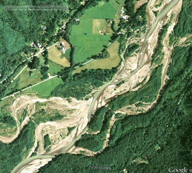
Here is the study area in 2005:
Here is the same area in 2009:
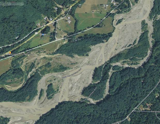
Note that some channel migration is apparent between these two images.
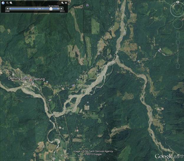
Here is an overview of the area:

Get the data: For starters, go to the Y-drive and grab this folder:
Y:\Courses\ESCI Wallin (442)\ESCI442_w2025\lidar_nooksack
Copy this entire folder to your working folder on C:\temp. It is quite large. Be patient.
Text
files vs. LAS files: Sometimes the all returns data are distributed at .txt files and
sometimes they are distributed as LAS files. LAS files are more compact and
more easily used by FUSION. It is useful to know how to convert .txt files to
LAS. So…..
Convert All Returns Text Files to LAS Format: Inside the \lidar_nooksack folder, you will find a \nook2005 folder. Inside this, the \all_returns_text contains the raw, all-returns data stored as ascii text files. Our first task will be to convert these files into the LAS format that FUSION can work with more efficiently. You will be working with data from 12 different “tiles:”
Open FUSION. From the main menu, go to Tools-Data Conversion-Import generic ASCII Lidar data. From the Import ASCII data dialog box, click on the upper Browse.. button and navigate to the \nook2005\all_returns_text folder and select the first of your text files, q48122g2124.txt:
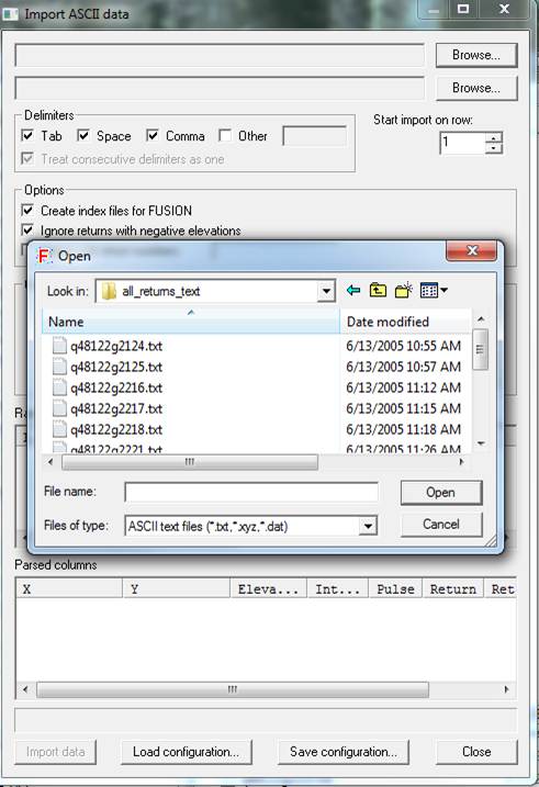
…and then click Open.
Now click on the second Browse… button and select a destination for the the .las file that you will create with this process. Put this file in your \nook2005\all_returns_las folder. You will note that there are already a bunch of LAS files there. This is because I’ve already created most of the LAS files for you, I’m just having you create this first one just so you know how to do it.
You will note that there is already a LAS file called
q48122g2125.las, so, you might just select this file and change this file name to q48122g2124.las. You just have to change the last number, the 5, to a 4.
Click Save to enter this selection
We will retain all the default settings under the Delimiters and Options section of the dialog box. Also, leave the Start import on row: set to “1.” The Column assignments section of this dialog box is critical! To guide you in completing this section, go back to the \nook2005 folder and open the “nooksack_nfork_2309_Final Report.pdf.” At the bottom of Page 7 of this report, you will find the information that you will need. The column assignments should look like this:
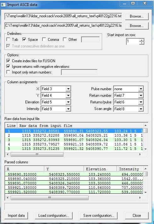
Note that the “Pulse Number” is not recorded in this data set (we don’t need this) and also that there are a few things in the dataset that will not be read in by this FUSION function (GPS Week, GPS Time and Classification Code). It is unfortunate that we can’t use the classification code. This designates whether a given point comes from the ground (G) or from vegetation (V). Not sure how the Lidar vendor determined this but it is interesting.
At this point, you should click on the Save Configuration button. This will enable you to save the field assignments so that you will not have to re-enter this for the subsequent text files that you will convert. You can store this configuration file anywhere within the \nook2005 folder.
Finally, click on the Import data button to import the data.
I have already converted the other 11 .txt files for you.
So you can move on.
Creating an Image file: Unfortunately, I do not have an image of this area that is clipped to the extent of the study area and FUSION requires an image. We can create a crude image of the study area by using the intensity data for each of our LIDAR data points. To do this, from the FUSION main menu, go to Tools-Miscellaneous utilities-Create an Image using LIDAR point data. From the resulting file Open dialog box, navigate to the folder that contains all of the .las files that you just created and select all 12 .las files (hold the control button down as you click on all 12 files) and click on Open. In the Image creator dialog box, click on the Browse button to select a destination (I’d suggest that you simply put this in the \nook2005 folder) and enter a filename (I’d suggest something simple like “nook2005”) and be sure to give the file a .bmp suffix! Leave all of the other settings unchanged and click on the Create image button. Be patient (a minute or so) until you see a “Done!” message, then close this dialog box.
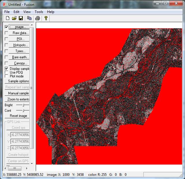
View the Data: Back in the main FUSION window, click on the Image button: and select the .bmp file that you just created. The image should appear in the main window. The display should now look something like this:
Now click on the Raw data button: and select all 12 .las files. This brings up the Data files dialog box. Leave everything unchanged here and hit OK.
At this point, and as you did in the LIDAR intro, you can push and hold the left mouse button to highlight a subset of the image and view the data with the LIDAR Data Viewer.
Using FUSION Functions from the Command Prompt: We now need to run some Fusion functions using the command line. This is a bit clunky and may seem quite primitive to those of you who are used to using the graphical user interfaces that are common to most computer programs. However, these command line functions are quite powerful and enable you to link commands to create scripts that will execute several commands in sequence.
Explore the data with the
Catalog command: Take a look inside the \nook2005\fusion_bat folder. Use a text editor (Notepad is a
good choice; just go to the Windows ![]() Search and enter “Notepad”) to open the
catalog.bat file. Refer to the FUSION manual (located in \fusion_tutorial\FUSION\doc) to understand the syntax of the
command and the meaning for the various settings. Then to the Windows
Search and enter “Notepad”) to open the
catalog.bat file. Refer to the FUSION manual (located in \fusion_tutorial\FUSION\doc) to understand the syntax of the
command and the meaning for the various settings. Then to the Windows ![]() Search and enter “Command Prompt”. You will really
only need to enter the first few letters and then you can just select “Command
Prompt.” This will bring up a box that looks like:
Search and enter “Command Prompt”. You will really
only need to enter the first few letters and then you can just select “Command
Prompt.” This will bring up a box that looks like:
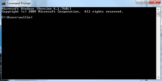
The first thing that you need to do is navigate to your \nook2005\fusion_bat folder. To do this, you will use the “cd” command in the Command Prompt window. Enter “cd ..” (note that there is a space between the cd and the dot dot; and, by the way, “cd” stands for change directory) to go up one level in the directory structure (to c:\Users from C:\Users\wallin in the above window). Then enter “cd ..” again to move to the root directory which is simply C:\ Then “cd folder” (where folder is the name of the folder that you want to move to) to start moving back down through the directory structure to get to your working directory. Enter “dir” (stands for directory) to see the contents of a given folder. Back in the olden days before Windows, commands like this were the ONLY way to interact with your computer! NOTE: to change from one drive to another (like from the c:\ drive to e:\ drive), use “cd /d e:\”
In my case, I want to navigate to C:\Temp\wallin2020\lidar_nooksack\nook2005\fusion_bat. From this location, simply enter “catalog” in the Command Prompt window to execute the catalog command. A bunch of stuff will scroll by in the Command Prompt window. When it is finished running, go to the \catalog_output folder (using My Computer, not the Command Prompt) and click on the .html file. This will provide lots of information regarding the Lidar point density. Take a look at everything. I have set up the catalog command to determine the return density in grid cells that are 2 meters by 2 meters. My desired total return density is 1 hit/m^2 (4 hits in each 2 m grid cell) and a first return density of 0.25 hits/m^2 (or at least one hit in each 2 m grid cell).
Creating
a Bare Earth Layer:
I. Groundfilter: With your text editor, open \fusion_bat\groundfilter.bat. Refer to the FUSION manual to understand the settings associated with the groundfilter command. Basically, what it does is to classify the individual points as either a ground return or a return from the vegetation. After familiarizing yourself with the command, go to the Command Prompt and enter “groundfilter.” As it starts to run a window will pop up that looks like this:
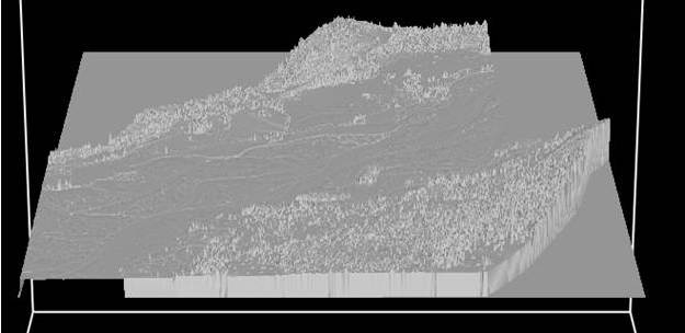
Note that up on the slopes away from the main channel, the land surface is “fuzzy” due to all of the trees sticking up. As the groundfilter functions runs, more and more of these returns from vegetation will be eliminated until only the ground returns are used to create the bare earth layer. The function isn’t perfect and a few vegetation returns will be incorrectly retained leaving spikes in the bare earth layer. Here is what my final bare earth layer looks like:

Better, but not perfect. If you’d like, you can play around with some of the settings in the groundfilter command (your groundfilter.bat file) to see if you can get a better result.
The groundfilter command yields a file, nfork2005_groundpts.lda, which is kind of like your starting .las files but it only includes the points that have been classified as ground returns. Although the data viewer (screenshot above) creates a visualization of the bare earth layer, this was a temporary file. We now need to create a final bare earth layer using our ground points file.
II. Gridsurfacecreate: Use your text editor to open \fusion_bat\gridsurfacecreate.bat. Refer to the FUSION manual to understand the details of this command. Then, in the Command Prompt window, enter the command, “gridsurfacecreate”.
III. View the Bare Earth Layer: Back in the FUSION window, click on the Bare earth button and select the \nook2005\nfork2005_surfact.dtm file. This brings up the Surface model dialog box. Take the default settings and click on OK.
In the main FUSION window, click on Sample options, and set the Decimation to include every 100 data points, then click OK. Select a subset of your scene to display. In the LIDAR Data Viewer window, right-click to bring up a bunch of options. When I turned on “Surfaces” and turn off “Data” here is what mine looks like:
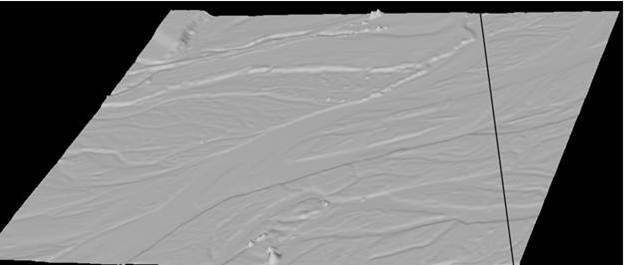
There are a few “dimples” from vegetation points that have been incorrectly retained in the bare earth model but it looks pretty good, at least within the active channel of the river. We have lots more to do so let’s move on.
Export your Bare Earth layer: You can refer to Exercise 5 in the tutorial for instructions on exporting your bare earth layer (so we can work with it in Arc). You can do this export from the Fusion main menu by clicking buttons, but ya know, it is easier to do this from the command line. With your text editor, open \nook2005\fusion_bat\dtm2asciisurface.bat. As you can see, there is not much to this command. So, in the Command Prompt window, enter “dtm2asciisurface”.
Canopymodel: We also want to create a “Canopy Model.” This is based on the 1st return from each LIDAR pulse and represents the top of the vegetation canopy. In parts of the study area with no vegetation, the bare earth and canopy models are identical. In your text editor, open the \fusion_bat\canopymodel.bat file. As before, refer to the FUSION manual to understand the settings associated with the canopymodel command, then execute this command from the Command Prompt window.
View the Canopy Layer: Back in the FUSION window, select a sample box over a forested part of the study area. In the LIDAR Data Viewer window. Right-click to bring up all of your options and select Surface file, then select your new nfork2005canopy.dtm file. You might also toggle your all returns data on and off to help you visualize the relationship between the canopy model and the all returns data. You will note that your canopy layer will be a bit below your highest points. This is OK.
Export your Canopy layer: As with your suface model, you want to export your dtm file to ascii format. Use the \nook2005\fusion_bat\dtm2asciicanopy.bat file to do so.
Repeat for the 2009 Data: OK, now we need to do nearly EVERYTHING that we did above for the 2009 data! But ya know, now that you are wizards with the use of FUSION commands and .bat files, we can make this really easy. Working with the 2009 data is a bit easier since we already have .las files. We don’t need to do the text file import to las files.
Using these .las files as a starting point, we want to run six different .bat files:
Catalog.bat
Groundfilter.bat
Gridsrufacecreate.bat
Canopymodel.bat
Dtm2asciisurface.bat
Dtm2asciicanopy.bat
I have already edited each of these files in \nook2009\fusion_bat so they are all set to run and you can launch all of them at one time. To do so, note that each of the six .bat files are there, but also note that there is another file called “six_full_cmds.bat.”
Open this file in your text editor, and take a look at it. It should look like this:
c:\temp\fusion\catalog /index /coverage /density:4,1,2 /firstdensity:4,0.25,2 /intensity:4,0,255 /bmp /outlier ..\all_returns_las\*.las ../catalog_output/nook2009_4
c:\temp\fusion\groundfilter /gparam:-1 /wparam:2 /tolerance:0.1 /iterations:15 /diagnostics ..\nfork2009_groundpts.las 6 ..\all_returns_las\*.las
c:\temp\fusion\gridsurfacecreate ..\nfork2009_surface.dtm 6 F F 2 WAN 2 2 ..\nfork2009_groundpts.las
c:\temp\fusion\canopymodel /smooth:3 ..\nfork2009_canopy.dtm 6 F F 2 WAN 2 2 ..\all_returns_las\*.las
c:\temp\fusion\dtm2ascii ../nfork2009_surface.dtm
c:\temp\fusion\dtm2ascii ../nfork2009_canopy.dtm
Note that there is one command per line.
In your Command Prompt window, navigate to \nook2009\fusion_bat and simply enter “six_full_cmds” (without the “”). This will take a few minutes, but this will execute each of these six commands one at a time. This does the same thing that would happen if you executed one command, waited for it to finish, entered the next command, waited for it to finish……and so on.
Pretty cool isn’t it!? This should give you an appreciation for the usefulness of the Command Prompt.
After everything finishes running, go to \catalog_output and look at the .html file to get a feel for the pulse density in this dataset. You can then load everything in the main FUSION window if you’d like to look at the bare earth layer.
We now want to bring both bare earth layers and both canopy layers into Arc to compare them to look for changes in channel morphology.
Import the 2005 Bare Earth Layer into Arc:
Start by opening ArcPro. Create a new project. From
the Map tab in the menu ribbon, select Add data ![]() and select your “nfork2005_surface.asc”
file…but note that to do so, you may need to change the data type from
“Default” to “Rasters (all local types).” Select
“Yes” when asked if you want to build pyramids.
and select your “nfork2005_surface.asc”
file…but note that to do so, you may need to change the data type from
“Default” to “Rasters (all local types).” Select
“Yes” when asked if you want to build pyramids.
Convert Ascii to raster: From the “Analysis” tab in the menu ribbon, select “Tools”. In the pane that pops up on the right side of your screen, search for the “Copy Raster” tool. Parameters for this tool should be:
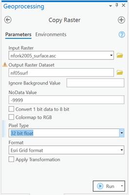
When specifying your output
Raster Dataset, don’t forget to click on the folder icon and specify the folder
where you are working!!!!!!!!!!!!!!!
Important Note: All raster grid file names in ArcPro
are limited to 13 characters!
Click “Run”
Define Projection: When you create this raster grid,
not projection information comes in with it. So we
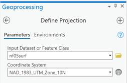
will need to fix this. Search for the “Define Projection” tool. Your input file
for this will be the “nf05surf” file that you just created. For “Coordinate
System” click on the little globe ![]() This brings up the Coordinate System diolog box. Go to Projected Coordinate Systems –North
America- UTM – NAD83 – NAD83 UTM Zone 10N. Then back in the Define
Projections dialog box, click Run.
This brings up the Coordinate System diolog box. Go to Projected Coordinate Systems –North
America- UTM – NAD83 – NAD83 UTM Zone 10N. Then back in the Define
Projections dialog box, click Run.
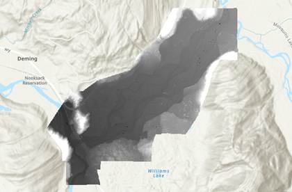
To double check if you did the “Define Projection” correctly, right click on the “nf05surf” layer in the contents pane on the left, click “Zoom to layer”. The raster should reload and be positioned over the Nooksack River near Deming, WA
Import the 2009 surface ascii file: Repeat steps above for the 2009 surface layer to convert from ASCII to Raster (“nfork2009_surface.asc”). But note that the 2009 data are in a different projection than the 2005 data. Navigate to the correct projection for the 2009 data using: Projected Coordinate Systems à State Plane à NAD 83 HARN (US Feet) à NAD_1983_HARN_StatePlane_Washington_North_FIPS_4601_Feet
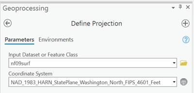
Convert from State Plane to UTM: Next, we need to reproject the 2009 data to match the 2005 data. Navigate to the “Project Raster” tool.
a. Input raster: nf09surf
b. Output raster: nf09surfutm (save to your nook2009 folder)
c. Output coordinate system: NAD_1983_UTM_Zone_10N (same as above, navigate to this coordinate system with: Projected Coordinate Systems à UTM à North America -- NAD83 à NAD83 UTM Zone 10N)
d. Output Cell Size: same as nf05surf (this will change the X and Y to 2)
e. Leave all other parameters as-is
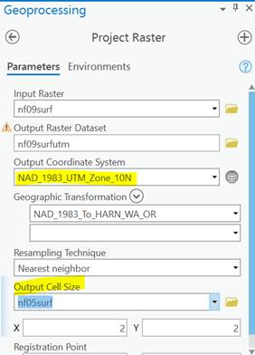
What did we just do? We just converted the 2009 layer from State Plane to UTM, clipped it to the same spatial extent, resampled it to have the same 2 meter grid cells as the 2005 layer (the 2009 layer had cell sizes of 6 feet coming out of FUSION) and also made sure that the grid cells in both layers line up perfectly. So, at this point, the 2009 and 2005 layers should line up perfectly. Try clicking them on and off to confirm. The only bummer here it that the 2005 layer extends a bit farther upriver than the 2009 layer but we can’t do anything about this.
Calculate Elevation Change Between 2005 and 2009 using the Bare Earth models? We can finally address the question that we started with. We can simply subtract the 2005 layer from the 2009 layer. One final annoying issue is that the elevations in the 2009 layer are in feet and the 2005 elevations are in meters (#@$#%!!!!). We can do the conversion (feet to meters) and the subtraction in a single step in the raster calculator. Search for the “Raster Calculator” tool (Note that the “Raster Calculator” is similar to “Band Math” that you have used in ENVI). Enter an equation like this:
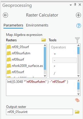
Notice the “Int” at the beginning of this expression. This is here to convert your results into integer values rather than floating point numbers (with decimal places). To insert this function, scroll down in the Tools window and double-click on it to select. And be sure that your Output raster name has no more than 13 characters in it!
Click “Run”
After the raster calculator finishes, you can right-click on the output and go to Properties-Symbology to create a cool color scheme (more on this discussed below). We have lots more to do and we’ll come back to this so let’s move on.
Import
the Canopy models: OK now repeat what you just did using the 2005 and
2009 bare earth models using the Canopy models. So, you will need to do
the Ascii to Raster conversions using the “Copy Raster” tool and fix the
projections. Review the steps above as needed
Calculate Elevation Change Between 2005 and 2009 using the Canopy models: OK, now subtract the 2005 canopy model from the 2009 canopy model just as you did for the bare earth models.
Just to add one more wrinkle, I’m also providing you with a digital surface model (a canopy surface model) and an ortho photo that were created using imagery from our unmanned aircraft. We will be discussing unmanned aircraft systems (UAS) next week and we’ll do a bit of show and tell in lab next week. Your \lidar_nooksack folder includes a \nook2016 folder. This contains three TIF files, two ortho images (one for Aug 30 and the other for Sept 1) and a Canopy model (sept1_2016_flts1_5_dem_utm.tiff). These are based on about 6400 images acquired over a two-day period. The ortho image has a pixel size of 4 centimeter! (no this is not a typo!) The canopy model has a pixel size of 16 cm. All three of these files are huge. The folder also includes a PDF with information regarding these files. These files are in UTM with elevation in meters for the Canopy model.
The folder also includes a shapefile called “Channel.” This layer defines the channel migration zone and a bit later, we will clip our difference layers using this file so that we can confine our elevation change analysis to just this zone.
Add all 4 files to
your Arc project. You will be asked
to create pyramid files and calculate statistics. You should say yes. These are huge files so it may take some
time to complete this!
The 2016 canopy surface model is equivalent to the 2005
and 2009 canopy surface models.
Canopy elevation change from 2009 to 2016: Use the raster calculator to subtract the
2009 canopy surface model (NOT the 2009 bare earth model) from the 2016 canopy
surface model. Don’t forget to correct for the fact that the 2009 elevation are
in feet, just as you did above.
Canopy elevation change from 2005 to 2016: Note that the extent of the 2016 and 2005
layers are larger than the 2009 layers. So, use the
raster calculator to subtract the 2005 canopy surface model (NOT the 2005 bare
earth model) from the 2016 canopy surface model. Both of these layers have
elevations in meters so no correction is needed.
Before
diving too far into interpretation, let’s do a reality-check. Take a look at the Ortho image from 2016. What feature(s) in
the study area would you expect NOT to change in elevation over this 11 year interval?
Think real
hard……..
How about
the roads? Yes, some of the roads might have been resurfaced but this would
only result in a change of a centimeter or two. And yes, there might be a few
places where there might be some slumping/subsidence
but this is likely to occur in only a handful of places.
So, let’s take a look. First, from
the Map tab in the menu ribbon, select Explore. Then Zoom in on a
section of road (with the 2016 ortho layer activated). With the Explore tool
active, when you click on a location in your map, a pop-up window will appear
that will display the elevation at that location. Use this tool to get the
elevation difference for this location for each
of your difference layers. Record this value by entering this into a
spreadsheet. Zoom out and move to
another part of the study area and try again. Repeat this for ~20 locations that
are well distributed around the entire study area (both sides of the river) and
then calculate the mean, maximum and minimum differences. From this, you should
see a systematic bias. One of the layers seems to be a bit higher than the
other. You can use your mean difference from your road points for bias correction (below).
But first,
which elevation layer is “wrong?”
In
reality, it doesn’t
matter for this analysis. We don’t need to know the “true” elevation for any of
these layers. We just need them to line up. So, I’m pretty sure that you noted
that the difference in road elevation between the 2005 and 2009 layers was
very, very close to zero. Plus or minus a few
centimeters; ~0.02 meters. However, you probably noted that, for the roads, the
2016 minus either the 2009 or 2005 layers was close to -1.0 m or a bit less.
So, this means that the 2005 and 2009 were about 1 meter LOWER HIGHER
than the 2016 layer. This is almost certainly due to an error in the vertical
datum that I used when defining one of the projections.
The easiest way to correct
for this systematic bias might be to simply ADD ~1 meter (or whatever you found
to be the mean negative difference) to each of the 2016 minus 2009 or 2005
layers using the Raster Calculator.
Zoom in on
some of the big losses and gains and see if you can figure out what is causing
them. To help you interpret this, toggle between the 2016-2005 elevation
difference, the 2005 shaded relief, and the 2016 ortho images.
What are the
drivers of these big (+ or – 10-20 m) losses and gains?
What is the
driver of the more modest (+ or – 1-2 m) losses and gains?
Note that
the maximum elevation loss is -352 m and the maximum
elevation gain is +67 m. Do these max/min values seem reasonable/realistic? Are
these values “real” or due to some anomaly in the data? What do you feel
represents realistic maximum elevation losses and gains? This would be a good
discussion point for your lab report.
Frequency Distribution of Change in Channel Migration Zone:
Some of the
area in our difference images is “upland” that is not within the channel
migration zone. We would like to quantify the amount and percentage of
the area within the channel migration zone has undergone different types of
change. I manually created a polygon
that approximately delineates the channel migration zone. Add the shapefile channel.shp to your project (click the ![]() button again and point to “channel”
in the same folder with all of your other input
layers).
button again and point to “channel”
in the same folder with all of your other input
layers).
We now want to clip EACH of our difference images using the “channel” polygon. To do this, once again go to Analysis tab in the menu ribbon, select “Tools”. In the pane that pops up on the right side of your screen, search for the “Clip Raster” tool. For each of the difference rasters tha you have created, clip them using the channel.shp file as the “Output Extent.” And, make sure to check the “Use Input Features for Clipping Geometry.” Like this:
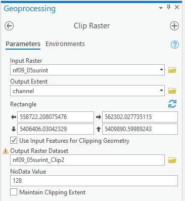
Display Symbology: It will be helpful to give your
elevation change layers a useful color scheme. To do so, right-click on one of
your elevation change layers in the Contents in Arc and go to Symbology. Select Classified and a Method of Manual. I’d suggest that you go
with 10 classes. I chose to use the following class breaks:
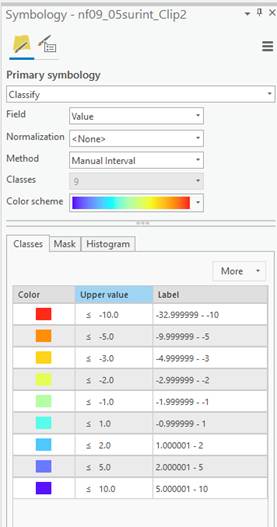
I selected a
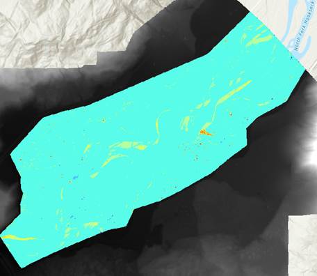
warm (red) to cool (blue) color scheme to represent elevation loss and gain,
respectively. My 2009 – 2005 surface layer looked like this:
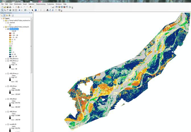
My 2016-2005
canopy elevation change layer looked like:
Frequency
distribution of elevation change: Finally, to generate a frequency distribution of elevation
change for each of your different layers, you can simply right-click on the
layer name in the Contents panel and go to the Attribute Table. There
are three columns in this table only two of which are relevant to us. The
“Value” is the elevation change values and the “Count”
is the number of pixels with each elevation change value. Click on the three
bars on the right side of this window ![]() and go to Export. For the
“Output Location” I’d suggest specifying a folder (not the *.gdb) and be sure to give your “Output Name” a *.txt suffix.
You can then open this text file in Excel and calculate the % of your study
area in each of the categories you used above when generating your symbology.
and go to Export. For the
“Output Location” I’d suggest specifying a folder (not the *.gdb) and be sure to give your “Output Name” a *.txt suffix.
You can then open this text file in Excel and calculate the % of your study
area in each of the categories you used above when generating your symbology.
Lab Report: With the loss of our Segmentation lab last
week, this is the 4th lab we have done this quarter for which you
could write a lab report. We will have one more lab next week (our 5th
not counting the Segmentation lab). For the Lab portion of the class, your
grade is based on your best 4 lab report grades. You have the option to elect
turn in only 4 lab reports (but, as discussed earlier, everyone was required to
turn in the Baker to Bay classification). If you are happy with your grades
thus far, you could elect NOT to turn in next week’s lab or you can turn in a
report for next week’s lab and drop your lowest grade.
If you choose to do
a report for this lab, you should discuss the elevation changes both the bare
earth (2005 to 2009 only) and the canopy surface models (2016-2009, 2016-2005,
2009-2005) time intervals. The bare earth models represent change ONLY in the
surface of the gravel bars but the canopy surface
models provide information about changes in the elevation of the gravels bars
(only in areas with no vegetation) and changes in the elevation of the top of
the vegetation canopy (in areas where there is vegetation). So, changes in the
canopy surface models tell you about the loss of vegetation (in the case of
negative values) or the growth of vegetation (in the case of positive values).
There is much to
talk about here!
Lab report due on either 2/25 or 2/26, at the beginning of lab
next week.
Return to ESCI 442/542 Lab Page
Return to ESCI 442/542 Syllabus
Return to David Wallin's Home Page