ESCI 442/542
Lab IV: Change Detection Using Unsupervised
Classification with ENVI
Outline of Document
(Click on links to jump to a section below):
Procedures:
Step
2: Unsupervised Classification
Step
3: Identification of Information Classes
Step 5: Masking out the Non-forest Areas
Step 6: Summarize Your Results
Last Updated: 2/10/2025
Objective: Conduct a Change Detection analysis using Unsupervised Classification to quantify rates and patterns of forest disturbance within a multiownership landscape. The basic procedures follow those that you used for the prior lab and will incorporate some methods from the Persian Gulf lab as well. I will challenge you to attempt these methods unaided when possible. Consult the web page related to these prior two labs for these processing steps when necessary. Our analysis will be based on imagery from 1988, 1992, 1995, 2000, 2005 and 2011. Your secondary objective will be to evaluate the effectiveness of the analysis and to support your claims with qualitative and quantitative evidence from your results.
Prior to lab, take a look at the following papers:
Cohen, W.B. et al. 1998. An efficient and accurate method for mapping forest clearcuts in the Pacific Northwest using Landsat imagery. Photogrammetric Engineering and Remote Sensing 64:293-300. cohen_etal_1998_apr_293-300.pdf
Cohen, W.B., T.A.
Spies, R.J. Alig, D.R. Otter, T.K. Maiersperger and
M. Fiorella. 2002. Characterizing 23 years (1972-95) of stand
replacement disturbance in western
And here is another nice Reference:
Whatcom, Washington, United States Deforestation Rates & Statistics: GFW.” Forest Monitoring, Land Use & Deforestation Trends, www.globalforestwatch.org/dashboards/country/USA/48/37/?map=eyJjYW5Cb3VuZCI6dHJ1ZX0%3D. Accessed 15 Feb. 2024.
Prior to lab, you should also read the section in your book that discusses the Tassel Cap Transformation of Landsat Data.
Introduction: As you know, Landsat I was launched in 1972 and so we now have an archive of imagery that spans 30 years. The availability of this long-term consistently acquired data set provides unprecedented opportunities to map and monitor land-use change. In the last lab exercise, you used Unsupervised Classification and Landsat Imagery to create a vegetation map for a single point in time for our Baker to Bay study area. For the current lab exercise, we use a series of six images to conduct a change detection analysis on this same study area. Our objective will be to quantify the rates and patterns of forest disturbance within this multiownership landscape. Most of the forest disturbance is in the form of timber harvest, but wildfires and windthrow also causes some disturbance. The study area includes a mixture of public and private ownership. Most of the private forest lands within the study area are owned by large corporations and these lands are intensively managed for timber production. The public lands are administered by the Washington State Department of Natural Resources and the US Forest Service. DNR lands are managed for multiple uses that include significant levels of timber harvesting. USFS lands are also managed for multiple use and historically, this included timber harvesting. Timber harvesting on USFS lands in our study area have been declining steadily since the early 1980s. The lands also include significant areas that are in congressionally designated Wilderness Areas and Recreation Areas that are off-limits to timber harvesting.
Procedures:
We have created nine .img files that contains all of the data needed for this lab. Each file is about 30 Mbytes. You will need at least 150 Mbytes of space somewhere to store the files needed for this lab. You should be sure to bring this with you to lab. The files you will need for this lab are in this folder:
Y:\Courses\ESCI Wallin (442)\ESCI442_w2025\
Files you need are in subfolders:
changelab\bbay_change2011_88.img
baker_bay_ENVI\imagery\bakerbay88.img
baker_bay_ENVI \ imagery\bakerbay92.img
baker_bay_ENVI \ imagery\bakerbay95.img
baker_bay_ENVI \ imagery\bakerbay2000.img
baker_bay_ENVI \ imagery\bakerbay2005.img
baker_bay_ENVI \ imagery\bakerbay2011.img
baker_bay_ENVI\bbay_elev_m.img
changelab\bakerbay_own_ENVI.img
Copy all nine files (both the .img files and the associated .hdr file; so really 18 files) to your personal workspace on C:\temp. A huge amount of work was involved in getting these files into their present form. These files were created using data from three Landsat TM images from the following dates:
August 10, 1992 (Landsat 5)
July 18, 1995 (Landsat 5)
September 25, 2000 (Landsat 7)
July 29, 2005 (Landsat 5)
July 30, 2011 (Landsat 5)
The 1995 image was carefully georectified to several reference maps. This involves locating easily identified ground features (e.g. road intersections) on the imagery and then shifting the imagery to line these features up with the “correct” UTM coordinates for these features. The “correct” UTM coordinates (based on NAD27) are obtained from the reference maps. The other scenes were then georectified to the 1995 image. This step is critical. If the images don’t line up properly, then many parts of the image will incorrectly be identified as “change.”
The next step in creating bbay_change2011_88.imginvolved generating images for each year that represent the Brightness and Greenness features of the Tasseled Cap Transformation. Briefly, each of these features represents a linear transformation of the six non-thermal TM bands. As you might guess, “Brightness” is a weighted index to the overall brightness of a pixel across the visible and IR portions of the EM spectrum. “Greenness” is an index to the amount of green vegetation in a pixel. It is created by primarily contrasting the DN values in the red and Near-IR portions of the spectrum. Why are these two indices useful?
As discussed in the Cohen et al. paper, forested pixels that have undergone a disturbance (timber harvest) are those that show an increase in brightness and a decrease in greenness from one year to the next. This spectral change occurs as the green conifer cover is replaced by logging slash and exposed soil. For sites where fire was used after timber harvesting to prepare the site for replanting, will be somewhat different. These sites will undergo a decrease in brightness (dark green forest to black fire residue) and a decrease in greenness. The critical step of course is to determine what magnitude of change in brightness and greenness represent a “real” change. We could use density slicing to determine this, but unsupervised classification will be a more objective and more elegant approach.
The “bakerbay88.img, bakerbay92.img, bakerbay95.img, bakerbay2000.img, bakerbay2005.img, bakerbay2011.img” files contain the TM bands 1-5 and 7 (the non-thermal bands) for each of these six years. These first three image files also contain the Tassel Cap indices. For the last three years, the tassel cap layers are in separate files (ranging in size from about 23-44 Mbytes). Don’t worry about these files for now. We will use these files a bit later when we get to the point of wanting to assign spectral classes to information classes.
The “bakerbay_own_ENVI.img” file, as the name suggests, includes an ownership layer for our study area. The file is about 3.7 Mbytes in size.
The “bbay_change2011_88.img ” is the main file we will be working with. It is about 148 Mbytes in size. You will be creating at least two additional files of considerable size before you complete your analysis. “bbay_change2011_88.img” contains the following data layers:
2011 Brightness minus 2005 Brightness
2011 Greenness minus 2005 Greenness
2005 Brightness minus 2000 Brightness
2005 Greenness minus 2000 Greenness
2000 Brightness minus 1995 Brightness
2000 Greenness minus 1995 Greenness
1995 Brightness minus 1992 Brightness
1995 Greenness minus 1992 Greenness
1992 Brightness minus 1988 Brightness
1992 Greenness minus 1988 Greenness
These ten difference images are what you will be using as a starting point for your unsupervised classification. The difference channels are just what the name implies. The first one was created by subtracting the 2011 Brightness index from the 2005 Brightness index. Note that these difference channels are stored as “floating point.” ENVI defines the “float” data type as a 32-bit (4 byte) signed channels. As 32-bit channels, they take up four times as much storage space as the 8-bit channels (ENVI defines these 8-bit layers as the “byte” data type) we have worked with in previous labs. 32-bit signed channels can store values ranging from –1 x 10^38 through +1 x 10^38. We don’t really need this full range of values but these difference images do need to be capable of storing positive and negative values so this is our only option. For more information on ENVI data types, from the ENVI main menu bar, go to Help-Contents, then in the search box, enter “IDL Tips”. View the information on all of the Data Types that are supported by ENVI.
Step 2: Unsupervised Classification. Following the procedure described in the previous lab, run an ISODATA Unsupervised Classification using these ten difference layers as input. I’d suggest that you use the same parameters (# classes, etc.) as in the previous lab.
Step 3: Identification of Information Classes. After ISODATA has finished running, your change class map will open in your existing view. This is a single band image containing the 50 change classes that were created by the ISODATA classifier. Your change layer it will open with a rather garish multicolor display. It will look something like this:
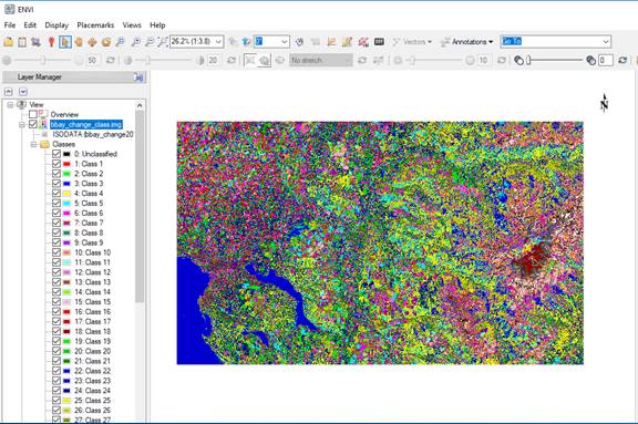
Each color
represents one of the 50 change classes that you requested. Your task at this point is to interpret this
image and assign each of these 50 change classes to one of our information
classes. Your objective is to
identify six Information Classes:
No Change
Timber harvest between 1988 and 1992
Timber harvest between 1992 and 1995
Timber harvest between 1995 and 2000
Timber harvest between 2000 and 2005
Timber harvest between 2005 and 2011
Use the visible images to help guide you in the process of identifying these information classes. To do this, it will be useful to be able to simultaneously view the same section of the change class image and the 1988, 1992, 1995, 2000, 2005 and 2011 images. This will enable you to identify areas that have been clearcut during each of our two time periods. You will also be able to identify areas that belong in our “no change” class. You have your change class image and images representing our six dates.
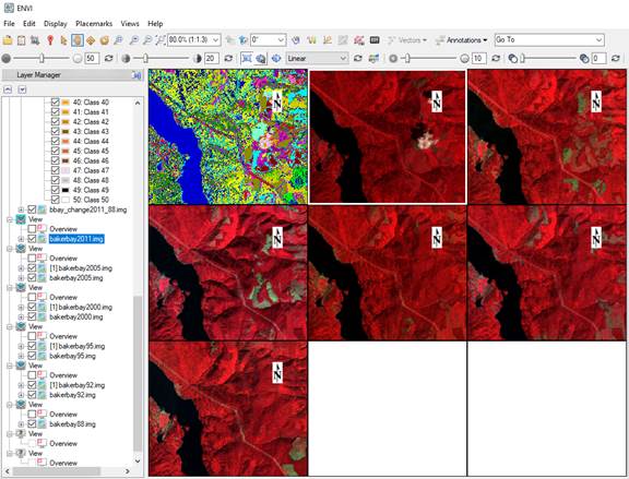
-In the main ENVI toolbar, go to Views-3X3 Views. We really just need seven views but 9 is our closest option. Your change class image should be in the upper left corner of your ENVI display, like this:
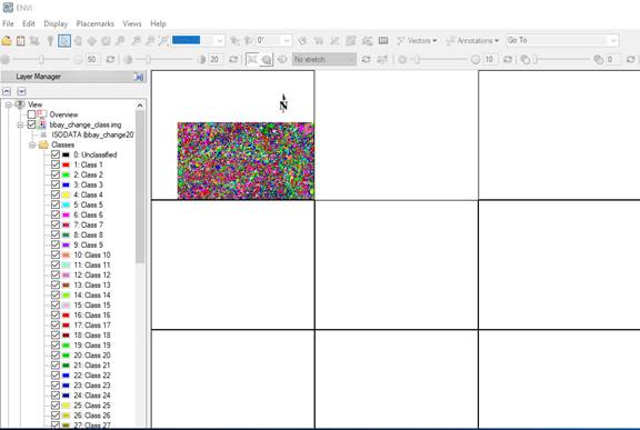
-In the Layer Manager window, click on the first view below the view that contains your change class image. This will end up being the view just to the right of the one containing your change class image.
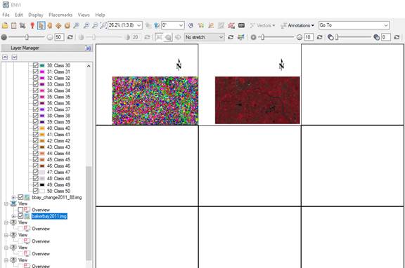
-Go to the Data Manager dialog and open your bakerbay2011.img file. Load this file as a color IR image into this view.
-In the main ENVI toolbar, go to Views-Link Views. In the Link Views dialog, select Link All, then click on OK. Your display should now look something like this:
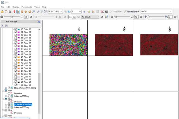
-Now move to the next view and in the Data Manager, open the 2005 image and load it as a color IR image into the next view. After once again linking the views, it should look something like this:
-Continue loading the images for the remaining four dates (2000, 1995, 1992, 1988) into the each of the next four views. After linking all of these views and zooming in on an area to the east of Lake Whatcom, your display should look something like this:
And here is the same image with some annotation added to point out some obvious clear cuts (timber harvest units) that have occurred during different time intervals.
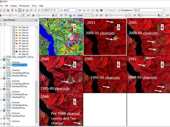
Unlike our previous lab, we do not have ground truth data to use to guide you in assigning change classes to our six information classes (listed above). However, simply viewing the images together should make it pretty simple to do so.
So, following the approach that you used last week, edit the class names and colors in your change class image to assign each of your 50 change classes to either the “No change” information class or to one of the five change class intervals. Note that most of your 50 change classes will be assigned to the “No change” information class. Pick a unique color to use for each of the six information classes (No change, 88-92 harvest, 92-95 harvest, 95-2000 harvest, 2000-05 harvest and 2005-11 harvest). For the class names, retain the “Class #” part of the name but add a descriptive name if you’d like (ex.: “Class 38: 88-92 change”). Assign all 50 change classes to one of the six information classes. Note that sites harvested BEFORE 1988 (obvious clearcuts appearing on the 1988 image) will go into the “No change” class. Most of the change classes will go into this “No change” class.
You will need to use your Cursor Value tool ![]() to
guide you in this process.
to
guide you in this process.
Step 4: Combining Classes: After you are confident of your class assignments and, as we did in the
previous lab, we will now create a simplified image which combines all change
classes that are in the same information class.
Instead of having 50 classes (many of which represent the same thing),
the resulting image would have only 6 information classes (no change, 88-92
harvest, 92-95 harvest, 95-00 harvest, 00-05 harvest, 05-11 harvest).
-In the Toolbox search box,
enter Combine Classes and click on this tool
-From the Combine Classes Input
File dialog box, select your “bbay_change_class.img”
(or whatever name you used for this file). Then click OK.
-In the Combine Classes
Parameters dialog box, for reasons that will become clear below, I would strongly suggest that you use the “Unclassified”
output class for your “No change” class.
All pixels assigned to this class will have a value of 0 and this will
be helpful in one of the later processing steps. You can use
output Class 1 for the “88-92 harvest” output Class 2 for the “92-95 harvest”
class…and so on. When creating this
output file, delete the empty classes and specify an output file name for your
combined classes image.
Load the file into a view and edit
the colors to the same ones that you used in your change class image. You should also edit the class names. Confirm that your change class image and
combined classes images look the same.
Step 5: Masking out the Non-forest, Agricultural lands and the High elevation areas.
Elevation Mask: Your change image will contain lots of change polygons that result from agricultural changes at low elevations and from year-to-year variation in snowpack at high elevations. You will now create a mask to take all change pixels above 1700 m ((but see note below)) and below 100m and reassign these to the “No Change” class. This will eliminate all change polygons above 1700m and below 100m. Note that you may decide to use different elevation cut-offs if you feel that it is appropriate.
NOTE: You should look at the image for 2011 and note that the
snowpack for this year on Mt. Baker is quite low. You should spend some time
determining the lowest elevation for this 2011 snowpack and use whatever value
you come up with when creating your elevation mask. 1700 m is probably much too
high.
You will create your elevation mask by following the same general approach that you used in the Persian Gulf lab.
You should have two views with nothing in them.
-In the Layer Manager window, click on one of these two empty views, then,
-In the Data Manager dialog, open the bbay_elev_m.img (this layer is in the J:\saldata\esci442\baker_bay_ENVI folder). Load this elevation layer in grey scale into your active view (one of the currently empty views.
We want to create a mask with all pixels in the agricultural zone and the alpine zone having values of 0 and all other pixels with a value of 1.
-In the Toolbox search window, enter Build Mask, then double click on the Build Raster Mask tool
-In the Build Mask Input File dialog, select “bbay_elev_m.img” then click OK
-In the Mask
Definition dialog, chose Options-Import
Data Range
- In the resulting Select Input for Mask Data Range dialog, first toggled Select By-Band. Then selected Layer_1 in the bbay_elev_m.img file and clicked OK.
- In the resulting Input
for Data Range Mask dialog, entered the min and max values that represent
our mid-elevation range (where we expect to encounter clear cuts; you might
start by using 100 to 1700 1400 m).
Pixels in this elevation range will get a value of 1 and everything above and
below this will get a value of 0. After selecting you elevation range, click
OK.
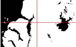
- Back in the Mask Definition dialog, selected an output path then entered an output filename for the output mask image. Then clicked OK. The result should look something like this, depending on what threshold value you chose:
Forest Mask: To create this mask, you will use the final classified
image that you created in the last lab using the 2017 BakerBay
image. However, for many of you, when you exported
this image from ArcPro, for some reason, and extra
row and column were added. Not sure why. Soooo, you
can use MY final map which you can find at:
Y:\Courses\ESCI Wallin (442)\ESCI442_w2025\baker_bay_ENVI\bbaaay17_final2
Also grab the .hdr file.
And yes, typo, I used 3 ‘a’s in the name. Sorry!
-In the Layer Manager, click
on your final unused view, then in the Data Manager dialog, open your
image classification from last week (your final product after running the
models in Arc). This file will have 12 classes.
-In the Toolbox search box,
enter Combine Classes and click on this tool
-In the Combine Classes Input
File dialog, select the file you just opened (final classification from
last week), then click OK
-In the Combine Classes
Parameters dialog, put all of your non-forest classes (residential,
urban, pasture, crop, water, rock, alpine, snow, shadow) into the
“Unclassified” category and put all of your forest classes (the clearcut, plus mixed and conifer) into
Class 1 (this will have the “Residential” label but don’t worry about this for
now). After doing so, click OK.
-In the Combine Classes Output
dialog, select “YES” in the Remove Empty Classes box, then select a
folder and filename for this (“forest_mask.img” might
be a good name) and click OK
Merge your elevation and forest mask: We now want to merge our elevation mask with our forest mask. To do so,
-In the Toolbox search box,
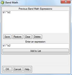
enter Band Math and click on this tool
-In the Band Math dialog and
the Enter and Expression window, enter “b1*b2” (without the “”) and
click OK
-In the Variable to Bands Parings
dialog we now need to define b1 and b2 by assigning data layers to each. Assign
your elevation mask to one and your forest mask to the other. It doesn’t matter
what order you choose.
-Choose a folder and filename.
Something like “elev_forest_mask.img” might be good.
What did we just do? In the
resulting data layer, everything above 1700 m and below 100 m (or whatever
thresholds you used) will have a value of 0. And, between these two elevation
ranges, all forest classes (clearcut, mixed, forest) will have a value of 1 and
all non-forest will have a value of 0. Run Quick Stats on your result to
confirm that your forest/elevation mask contains nothing but 0’s and 1’s. (Note
added 2/12/2020: After creating your forest/elevation mask, you may run
into ENVI standard file, ENVI classification file issue. See the info in the 3rd
paragraph down from here for instructions on dealing with this. You can import
header info from either your elevation mask or your forest mask.)
Using Image Arithmetic to Mask out non-forest, agriculture and high elevation land from your Change Map. After to come up your forest/elevation mask (mine is called elev_forest_mask.img) that you are happy with, we are ready to multiply your combined change image (mine is called bbay_ch_cl_comb2019.img) by this mask.
Again, the multiplication is done by using the Band Math tool in ENVI. You should be pretty familiar with this process by now so I will skip the step-by-step for this part. Refer to the instructions above if you need to.
ENVI standard file to ENVI classification file type: After completing this Band Math process, you will run into the same problem we faced last week when we opened the file we create in Arc in ENVI. The file is an “ENVI standard” file type and it displays in grey scale. In the Layer Manager window, the filename looks like this:
![]()
Note the grey window to the left of the filename. We need to edit the metadata for this file as we did last week. To do so,
-Right click on the filename and go to View Metadata. In the View
Metadata dialog, click on Edit
Metadata
-In the Edit ENVI Header dialog, click on Import ![]()
-In the Data Selection dialog, select your
combined change image. Mine is called “bbay_ch_cl_comb2019.img”. Note that, in
the Data Selection dialog, there is
a multicolored box next to the filename ![]() .
This indicates that this file has a file type of ENVI Classification rather
than an ENVI Standard file. After selecting this file, click OK
.
This indicates that this file has a file type of ENVI Classification rather
than an ENVI Standard file. After selecting this file, click OK
-In the Import Metadata Items dialog, select “Class names, Class colors and Number of classes”. Then click OK
-Wait a moment, then scroll down in the Edit ENVI Header dialog and you will now see the Class Names and Class colors info. Click OK to close this dialog box.
You will now see a multicolored box next to the filename in
the Layer Manager window. ![]() This
indicates that the file type has been changed to an ENVI Classification
This
indicates that the file type has been changed to an ENVI Classification
Your masked and
unmasked change images should now look the same, except that the low and high
elevation areas will appear black (assuming you assign black to the data range
from 0 to 0).
Eliminating small change polygons: You will notice that your change map includes many very
small patches of change. Most of these
probably do not represent “true” harvest polygons. They might represent small patches of trees
killed by insects or disease or errors due slight miss-registration of the
images from different years. We would
like to remove these from our map. Since
our focus is on identifying timber harvest, we can remove patches that are
smaller than a “typical” timber harvest unit.
For our purposes, we will delete all harvest patches that are smaller
than 2 hectares in size. Most harvest
patches are probably closer to 10 hectares at a minimum
but we’ll go with a 2 hectare minimum anyway.
Since our starting imagery had a pixel size of 25m by 25m, this involves
deleting all clumps of “change” that are less than 32 pixels in size.
We will remove these using “sieve”
and “clump” functions in ENVI.
-From the Toolbox search window,
enter Sieve. Double-click on
the Sieve Classes tool
-In the Data Selection dialog ,select your masked,
combined-classes image.
-This brings up the Classification
Sieving dialog box. In the Class Order window, select your five
harvest classes (you will need to hold down the CNTRL key to select all five of
them).
-In the Minimum Size box, enter
32.
-Leave the Pixel Connectivity box set at 8.
(If this is set to 4, then pixels that touch only at their corners don’t
count as member of the same patch [from chess, this is referred to as the
“rook’s rule”]. With a setting of 8,
pixels that touch on either a long edge or a corner are counted as members of
the same patch [again from chess, this is referred to as the “queen’s
rule”].)
-Specify an output folder and file
name and click OK. When you view the
result, you will note that all of the small change
polygons have been recoded to the background value of 0. This is why I suggested that you use a value
of 0 for the “No change” class.
You will note that many of the
change polygons appear somewhat ragged around their edges
and some have small inclusions of “No change” embedded within the change
polygon. You can address this by using
the “clump” function in ENVI.
- From the Toolbox search window,
enter Clump and click on the Clump Classes tool
-In the Data Selection dialog for this tool, select the file that you just
created using the Sieve tool. Then click OK.
This tool is a bit hard to
understand. So, in the main ENVI toolbar, you might want to go to
Help-Contents, then in the Index, enter Clump and read about it. Briefly, it
works by passing a majority filter over the image. The default is to use a 3 pixel by 3 pixel smoothing window.
This does a good job of smoothing out the image and recodes small isolated patches to the value of the majority of the
surrounding pixels. This may still leave
some “black holes” in your image since some of the larger patches are retained
by the clumping. If you’d like, you can
experiment with using a larger smoothing window; perhaps 5 by 5 or even 7 by
7.
-In the Classification Clumping dialog, and the Class Order window, select your five change classes. For starters,
you can stick with the default values of 3 for both the Dilate Kernel Value and the
Erode Kernel Value. You may choose to come back and re-run this with a
larger value.
-Select an output folder and
filename, then click OK
Step 6: Summarize your results. What is the amount of harvest (hectares) for the study area during each of the two time periods? Note that the length of each harvest interval is different (ex. 88-92 vs. 92-95). You can obtain this information by right-clicking in the display window and going to Quick Stats. Recall that the “Count” column in the Quick Stats output is the number of pixels. You can calculate area in hectares from this.
I would also like you to calculate the harvest rate on the basis of the % of forested area harvested per year (and note that each interval has a different number of years, ex 88-92 vs. 92-95 vs. 2005-2011). Calculating harvest rate on the basis of % of forest area is really more meaningful than the % of the total study area harvested per year. To get the total forest area, you will need to refer back the Forest_Elev_Mask that you created in Step 5 (above). Just go to this image and use Quick Stats to get the total forest area.
Finally, I would like you to calculate the % of forested
area harvested per year for different ownership categories. To do this, you will need the land ownership
layer in the file bakerbay_own_ENVI.img that is located in
J:\saldata\Esci442\changelab). The
study area includes four primary land ownership/management categories, each
with a unique numeric code in the bakerbay_own_ENVI.img
file. These are:
2 – Wilderness Areas
3 – National Forest
4 – Private Lands
5 – Dept. of Natural Resources
One easy way to use this is to go to Basic Tools-Band Math from the ENVI Main Menu. Create an expressing like this: (b1 *10) + b2. Then map b1 to the land ownership layer and b2 to your harvest map. This will yield an output image with values of 20, 21, 22, 23, 24, 25 that correspond to wilderness areas that are no change, 88-92 harvest, 92-95 harvest, 95-00 harvest, 00-05 harvest and 05-11 harvest, respectively. Similarly, the values of 30-35, 40-45 and 50-55 designate these six categories in the National Forest, Private lands and Dept. of Natural Resources, respectively. Pretty cool isn’t it?
OK then the final thing that you need to do is to come up with a denominator to use when calculating the ownership-specific harvest rates. To do this, we need the area of forest in each ownership category. To get this, you will need to do another Band Math operation using this expression: (b1 *10) + b2. Once again, your bakerbay_own_ENVI.img layer will be b1. But now, you will use your forest/elevation mask for b2. After running this band math operation, do a Quick Stats. The values 20 and 21 represent the non-forest and forest, respectively in the Wilderness. The values 30 and 31 represent non-forest and forest in the National Forest…..and so on.
Return to ESCI 442/542 Lab Page
Return to ESCI 442/542 Syllabus
Return to David Wallin's Home Page