ESCI 442/542: Introduction to Remote
Sensing
Last Updated 1/9/2024
Login Procedures: Hopefully, each of you now have your own personal functioning account in AH16. If you do not, getting one is the first order of business. Please take care of this prior to our first lab. Contact Dave Knutson in AH24 if you have problems.
Lab 1, Part A: Searching the Internet for
Imagery
Objective: This lab is intended to provide you with a taste of the Remote Sensing resources that are available on the web. We are going to accomplish the following:
o
Prepare a VERY brief memo using Word—or some
other word processing package.
o
Find a
way to "cut" a piece of your display screen and save it to a
file. Sometimes when you have an image displayed, you can simply
right click to save a copy of it to a file (there are many file extensions
and not all software accepts them all but the .bmp and .jpg extensions are usually a safe bet
for insertion; in general, .jpg files are smaller than .bmp files). If
the right-click option doesn’t work, there are several programs that allow you
to capture some or all of what you see on your screen. The program Hypersnap (located under Start-Programs) is one option. I
prefer the Snipping Tool (Go to
Start-All Programs-Accessories to find it).
o Search the Internet for an interesting remote sensing site and "capture" or save an image and paste it into your MS Word Memo.
Procedure:
- Spend some time surfing my List of useful Remote Sensing Links to get a feel for the variety of satellite imagery that is available. Alternatively, use http://www.yahoo.com or http://www.google.com and search the Internet on your own for sites related to this course---use words like "remote sensing," "space images"…….note when an http site name is highlighted in a Word document (and you have an internet connection) all you have to do is click on it and it will automatically open the site.
- Practice using the "capture" option of Hypersnap and/or Snipping Tool--annotate or modify it--save as a .jpg file.
- Create a VERY brief Word memo: describe the site, insert your image and caption it. Your memo should also include the image you will create in ENVI using the procedure describe in PART B of this lab (see below).
Lab I: PART B: Getting Acquainted with
ENVI
Objective: This lab is intended to introduce you to the ENVI image processing software that we will be using throughout the remainder of the course.
Preliminaries: You should begin by reviewing my suggested WORKING GUIDELINES before you begin. Following these guidelines will save you a great deal of time. After logging on, start My Computer to explore the directory structure a bit. As described in the Working Guidelines, the only place on the hard drive (c:/) where you have write permission is in the c:/temp subdirectory. Everyone can write files to this space. This is intended as working space and it is NOT intended for long-term file storage. In fact files stored here can be deleted by any user at any time. If you need more work space and if c:/temp is full of someone else's junk files, you have every right to delete them. Since we will be working with very large files, you should get in the habit of deleting your junk files before you log off. When logging on, it is a good idea to get in the habit of checking to see how much free space is available on the system. To do this in My Computer, click on the c:/ drive and go to File-Properties. There should be at least one Gbytes of free space. If there isn't, go to c:/temp, before you have opened any other applications, and start deleting files. You may not be able to delete subdirectories created by others under c:/temp, but you will be able to delete all files in these subdirectories.
Getting the Image:
·
In the Baker_Bay_ENVI folder, locate
the file called bakerbay2018.img. This is an image from July 8, 2018. Also grab
the bakerbay2017.img file. This is an image from August 22, 2017. Important Note:
the Microsoft Windows operating system may be confused by many of the files
that we use this quarter. Windows tries
to figure out what each file is and give it a “Type.” On my computer, all *.img files are
designated as WinZip files. This is
incorrect! If you see a bunch of WinZip
files and no *.img files then this is the problem. Just assume that the WinZip files are really
*.img files. Copy the file
bakerbay2018.img to your c:/temp subdirectory.
You may also want to put a copy of this file on your personal
storage space (Onedrive and USB drive). You will be working with the copy of
the image that you have placed in c:/temp.
Viewing a LANDSAT Image
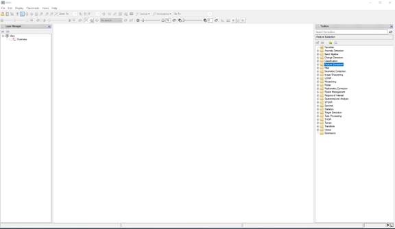
Start the ENVI software: Go to Start-All
Programs-ENVI5.7 and select ENVI5.7. Note that if you just go to Start-Programs
and select ENVI 5.7 Classic (or any that include IDL)you will get a completely
different interface. My instructions assume that you are using the new
interface. After opening ENVI, you will
see an interface that looks like this:
Opening an Image File
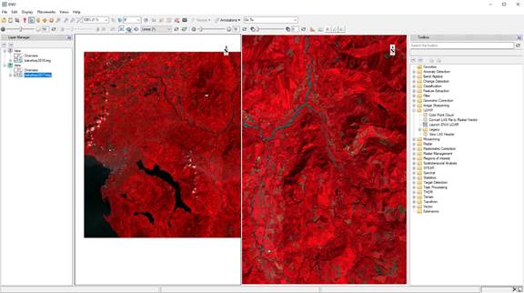
At this point, we would like to use ENVI to view our bakerbay2018.img file. To do this, from the main menu bar, go to File-Open Image File. Then navigate to the folder containing the bakerbay2018.img file, select the file and hit Open. It will look something like this:
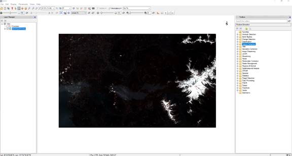
Boring at this point. Be patient.
Metadata:
Let’s start by looking at the details for this image by right-clicking on the image name and going to View Metadata. This will bring up this
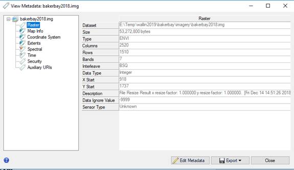
Feel free to explore the various tabs, then close this dialog box.
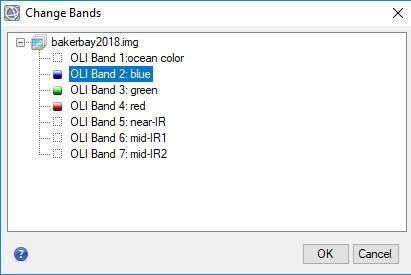
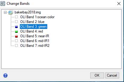
Now right-click on the image name and go to Change RGB Bands to bring up the Change Bands dialog box:
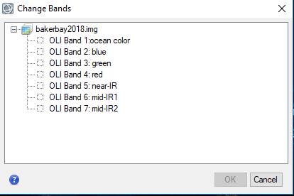
As you can see, this image consists of 7 bands that record the surface reflectance in different parts of the Electromagnetic spectrum.
Displaying the image
We can display a single band to produce a gray-scale image or multiple bands simultaneously as a color image. Your computer monitor displays images by mixing colors from three color “guns;” red, green and blue. We can display our satellite image by displaying one band using the red color “gun,” another band using the green color “gun” and a third band using the blue color “gun.” This is referred to as an RGB display. As we will see, different band combinations provide different sorts of information.
“True Color” Image:
Let’s start by creating a “true color” image. To do so, in the Change Bands dialog box, click first on “OLI Band 4: red.” When you do so, you will note that the little box to the left of the band name turns red, indicating that this band will be displayed using the red color gun in your video display. Next click on “OLI Band 3: green” and you will note that this will be displayed using the green color gun. Finally click on “OLI Band 2: blue” to display this band using the blue color gun. It should now look like this:
Click OK and your main display will now look like this:
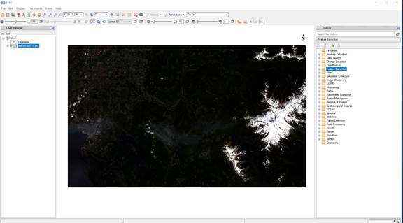
The image will look a bit dark. You can apply various “enhancements” to change the appearance of the image to bring out various details. Do this by click on the enhancements box here:
I found that the “Square Root” transformation looks pretty good:
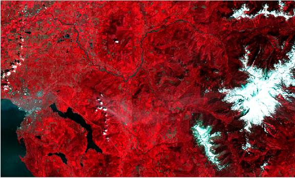
Color IR Image:
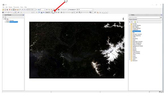
Let’s try another way to display the image. As you now know, vegetation is highly reflective in the near infrared portion of the EM spectrum. So, go back to the Change Bands dialog box and assign the Near-IR, red and green bands to the red, green and blue color guns, respectively. Like this:
Click OK and, using the “Linear 5%” enhancement, you should see this:
Viewing Single Bands:
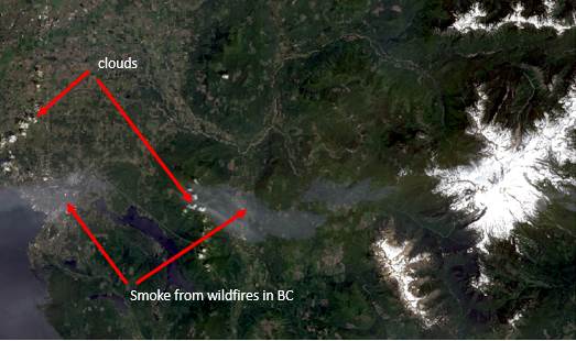
It is sometimes useful to view bands individually. One way to do this is to go to the very top of the ENVI window and select Display-Band Animation-Using Raster Series. This will begin displaying each band one at a time in grey scale and frantically cycling through them. Hit the pause button at the bottom center of the Band Animation dialog box, then click on the slider to examine each band one at a time. You will note that, in the first four bands, the image is fairly dark. When you go to band five, things get very bright. Why? Now go to bands 6 and 7 and note the appearance of the snow on Mt Baker compared to the clouds down near Lake Whatcom and to the north of Bellingham. You will note that the snow on Mt Baker and the clouds, are very bright for bands 1-5. However, in bands 6 and 7, the snow is very dark but the clouds are still very bright. This is one illustration of how different parts of the EM spectrum can be used to distinguish between different image features. Pretty cool isn’t it!
OK, now close the Band Animation dialog box and your display will go back to your color-IR display.
Other things to try
If you haven’t already discovered this, you can zoom in on the image just by moving the little scroll-wheel on your
mouse. Clicking on the hand icon ![]() enables you to move around the image. And feel
free to explore some of the other buttons.
enables you to move around the image. And feel
free to explore some of the other buttons.
Measurements: If you look to the north of Bellingham and zoom in a bit, you will find Wiser Lake, just south of the Nooksack River. It will look like this:
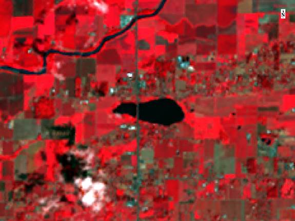
Pixel Size: The line that crosses the lake from north to south, just to the left of the center of the lake is Guide Meridian Road. At this scale, the appearance of the image is degraded and you can see the individual “pixels” that make up the image. The pixels in this image are 25 meters by 25 meters in size. (NOTE: A “standard” Landsat image has a pixel size of 30m by 30m. In your image, we have resampled the standard Landsat image to yield a pixel size of 25m by 25m. We’ll talk about how this is done later in the quarter.) When you start to work with any imagery, one of the first things you want to determine is the pixel size. In ENVI, you can obtain this information in the metadata (under map info).
Knowing the pixel size will give you a sense of scale and will be essential for enabling you to calculate areas and distances in your image. Just for fun, what is the maximum width (east-west) and length (north-south) of Wiser Lake? You can determine this by counting pixels and multiplying the number of pixels by 25.
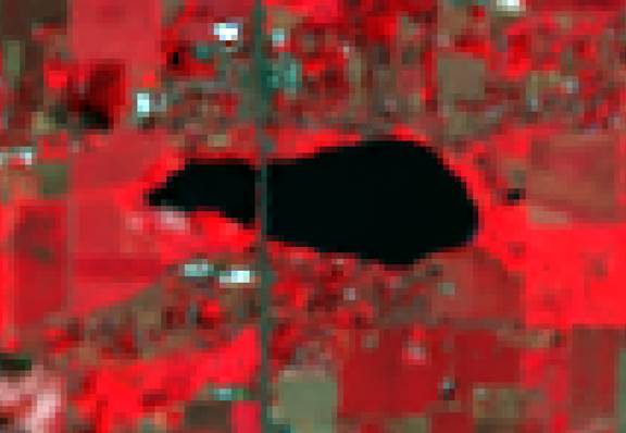
Measurement tool: OK, there IS an
easier way to get distances from your image.
Click on the measurement tool icon near the top of the window ![]() . Point to one end of the lake, left-click,
then point to the other end of the lake and left-click again. The Cursor
Value window will appear and you will see that the lake is about 1300 m
from east to west.
. Point to one end of the lake, left-click,
then point to the other end of the lake and left-click again. The Cursor
Value window will appear and you will see that the lake is about 1300 m
from east to west.
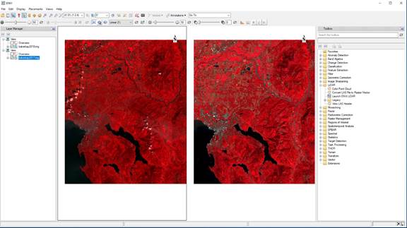
Comparing two images:
It will often be useful to be able
to view and compare two or more images. To do so, Views-Two Vertical Views.
In the Layer Manager window, click
on your second view, then up above, go to File-Open and open
bakerbay2017.img. This will bring up the Data Manager dialog. As you
have done for the 2018 image, load the 2017 image as color-IR, bands 5, 4, 3 in
the red, green and blue color guns, respectively. It should look something like
this:
On the left is your 2018 image and a
zoomed in subset of the 2017 image is on the right. It will be useful to link
the views so we are looking at the same location and at the same zoom level in
both views. To do this…..
Linking views:
Go to Views-Link Views to
bring up the Link Views dialog. Select Link All, then OK. You will see something like
this:
With the images linked, zooming in
one image does the same thing to the other. You can roam around the image to
compare them. One of the most obvious differences is up on Mt. Baker.
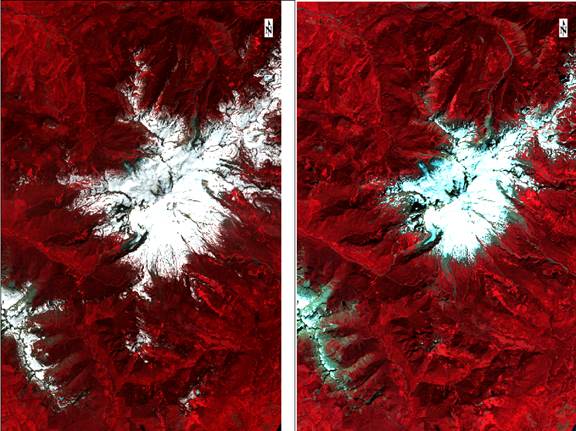
There is a big difference in
snowpack. The image on the left is from July 8, 2018 and the image on the right
is from August 22, 2017. Most of the difference here us just due to time of
year.
Feel free to play around with the
software.
Output: Follow the instructions above (in Part A) to use SNAGIT or the Snipping Tool to capture a true color and IR version of this Landsat image.
What you need to turn in: As stated above, there is no formal lab report required for this lab. You are required to turn in a memo created using MS Word that includes: a) the image you found on the Internet along with a brief caption describing the internet site and the image and; b) a “true color” version of the Baker to Bay Landsat image that you modified using ENVI and; c) an “Infra-red version of the Baker to Bay Landsat image that you modified using ENVI. Be sure to include a brief legend (aka “caption”) for each of the three images. Note: For this assignment and all lab reports for the class, you do not need to turn in a hard (paper) copy. Simply submit the file on Canvas to Bo or Anne (the TAs for the class; their email addresses are listed on the syllabus).
Return to ESCI
442 Lab Page
Return to ESCI
442 Syllabus
Return to David
Wallin's Home Page