Lab VII: Evaluation of
recreational impacts on eelgrass using UAS and virtual ground truth data
Last updated 2/26/2025
Objective: This
lab will involve the use of imagery acquired using a multispectral camera
carried by an Unoccupied Aerial System (UAS) to evaluate the impact of
recreational activity on eelgrass (Zostera sp.). This will involve the
use of regression analysis and “virtual” ground truth data.
Eelgrass (Zostera sp.) provides a
variety of important ecosystem services including stabilizing sediments,
buffering storm surge and nutrient filtration. It also provides critical
habitat for salmon, crab, shellfish and seabirds. Recreational impacts from
boat traffic, docks and mooring have been shown to have adverse effects on
eelgrass. Boat propellers can cut or uproot the vegetation and turbulence from
propellers can resuspend sediments generating turbidity and shading of the
vegetation and smothering as the sediment settles. Chemical pollution from
fuel, lubricants and anti-fouling paints can also have impacts. Docks can
impact eelgrass due shading and altered hydrodynamics resulting in erosion and
sediment translocation. Anchoring and mooring create mechanical damage to
vegetation and also stir up sediments. Two species of
eelgrass occupy the inland waters of the Pacific Northwest: Zostera marina and
Zostera japonica. Z. marina, the
native and most abundant species, is found in mid to sub tidal regions and Z. japonica, a non-native species, is
less abundant and is found in upper to mid-tidal ranges. Z. japonica is believed to have reached North America from Japan in
the packing materials of clam exports.
Traditional methods for monitoring
eelgrass involve the use of ground-based surveys that are quite time consuming
and limited in spatial extent. Imagery from satellites and traditional aircraft
have also been used but these approaches can be expensive, lack sufficient
spatial resolution and timing image acquisition to tidal cycles can be
problematic. More recently, the use of imagery acquired using low-cost,
unoccupied aerial systems (UAS) has been used. The advantage of UAS imagery is
the low cost, very high spatial resolution (a few centimeters) and ease of
timing image acquisition to tidal cycles.
Previous effort to monitor eelgrass using
UAS imagery has primarily been limited to simply mapping the presence or
absence of eelgrass without quantifying percent coverage or biomass. One recent
study was successful in distinguishing between Z. marina and Z.
japonica but only broke out four broad percent cover categories.
The objective of this exercise to evaluate
the use of simple vegetation indices, derived from multispectral imagery
acquired using UAS, in conjunction with a novel approach for obtaining ground
truth data, to quantify variation in the percent cover of eelgrass and to
evaluate the effect of recreational boat launch activity on eelgrass.
Study Area: Our study area for
this exercise is Wildcat Cove. Wildcat Cove is part of Larabee State Park (just
south of Bellingham) and it includes a boat ramp that
is heavily used during the summer months, particular during the recreational
crabbing season that typically opens in mid-July. During low tides, much of the
cove is exposed mudflat and vehicles typically back down across the mudflat to
get boat trailers to the water’s edge. Those launching kayaks and other
human-powered boats may also drive across the mudflat to the water’s edge. This
activity has an impact on eelgrass.
Preliminaries: As usual, go to
the Y-drive:
Y:\Courses\ESCI Wallin(442)\ESCI442_W2025\
And grab the entire “eelgrass” folder.
This folder includes imagery from two different date; July 14 was the Friday
before the opening of recreational crabbing season and July 17 was the Monday
after.
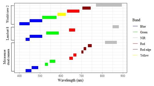
The data: We will be using
data collected using the Micasense Dual Camera
system. This is a 10-band camera. Here is how the bands on this camera compare
to the sensors on Landsat 8 and Worldview 2.
And here are the specifications for each
band.
Table 1:
Band
names, numbers, center wavelengths, and wavelength ranges of the Micasense Dual Camera System. The names, center
wavelengths, and numbers will be used in further writing in the format Band
Name Center Wavelength (Band Number).
|
Band Name |
Band Number |
Center Wavelength (nm) |
Wavelength Range (nm) |
|
Coastal Blue |
1 |
444 |
430-458 |
|
Blue |
2 |
475 |
459-495 |
|
Green |
3 |
531 |
524-538 |
|
Green |
4 |
560 |
547-574 |
|
Red |
5 |
650 |
642-658 |
|
Red |
6 |
668 |
661-675 |
|
Red Edge |
7 |
705 |
700-710 |
|
Red Edge |
8 |
717 |
711-723 |
|
Red Edge |
9 |
740 |
731-749 |
|
Near Infrared |
10 |
842 |
814-871 |
I’ve done quite a bit of prep work for you.
Each flight generated several thousand images. The “eelgrass” folder includes
two PDF files that describe each flight and the processing that was done that I
did to generate an orthomosaics that cover all of Wildcat Cove. I also
georectified the imagery with several ground control points located around the
perimeter of the cove.
View the imagery: Start by opening
“Wildcat_7_14_mica_60m_GCP_5cm_clip” in ENVI. This is a 10-band tiff file and,
as the filename suggests, the pixel size is 5 cm and
the imagery was obtained by flying at an altitude of 60 m above ground level
(AGL). There is an equivalent file for July 17, “Wildcat_7_17_mica_40m_GCP.”
This has a pixel size of 2.5 cm (I neglected to include this in the file name;
sorry) but I flew at 40 m AGL instead of 60 m.
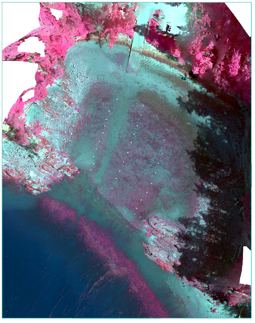
To view a color-IR image, you will need to
go to Change RGB bands and load bands 10,6,4 into the red, green and blue
color guns. You may need to try a few enhancements to brighten it up a bit. It
will look something like this.
You could also display a true color image
using one of the red, one of the green and the blue band (6,4,2). And, you can also view the image for July 17. Note that, in
addition to the high-resolution images for each date, there is
are also versions that have been resampled to generate images with a
pixel size of 50 cm. More on this below.
You will note the tide was quite low when
I did this flight and there is an extensive exposed mudflat covering much of
the cove. The red stuff on the mudflat, and in the water at the mouth of the
cove, is mostly eelgrass but there is also some algae
as well. You will also note a bare path from the boat ramp to the water’s edge
that is caused by people backing cars and boat trailers down to the water. Our
goal here is to assess the impact of this activity on the eelgrass after a
weekend of high activity associated with the opening of crabbing season.
Virtual Ground Truth: The three rows of
white dots (or squares if you zoom in) are ground control panels that I laid
out prior to my flight. The panels are spaced ~5 m apart and the spacing
between each row is ~15 m. These panels were used to generate “virtual” ground
truth data that we will use for the analysis. Prior to my flight to obtain this
imagery, I also flew quite low, just 5 m AGL, over these panels an took a
standard color image of each panel with a 20-megapixel RGB camera. I then
brought these images into Powerpoint and superimposed
a 4 by 4 grid adjacent to each panel. The panels are 45 cm by 45 cm and I resized the 4 by 4 grid to match the size of the
panel. This ensures that I was sampling a consistent area adjacent to each
panel. The cover type was visually assessed at the corner of each grid cell,
resulting in data for 25 points within this 45 cm by 45 cm sample grid. Percent
cover for each cover type was then calculated for each sample grid based on
these sample points. The four cover types included eelgrass (Zostera sp), algae (Ulva sp., mostly Ulva
intestinalis), bare and detritus. I did not distinguish between the two
species of eelgrass. Detritus is mostly composed of dead eelgrass.
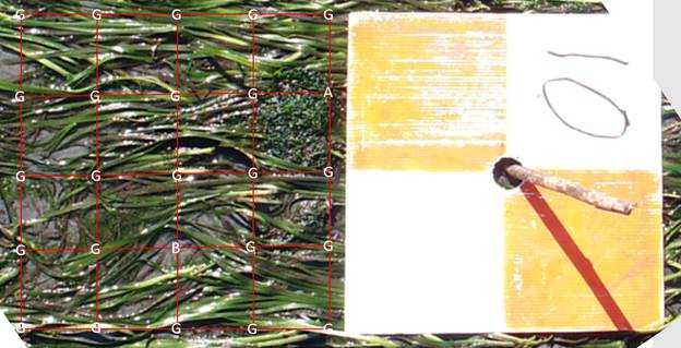
Here is an example of one of the “virtual” ground
control panels taken from just 5 m AGL with 4 by 4 sample grid superimposed on
the image. The cover type at the corner of each grid cell, was recorded and the
percent coverage of each cover type was calculated for the grid. The four cover
types included eelgrass (G), algae (A), bare (B) and detritus (D). Note that
detritus was not present at this location.
A typical approach for obtaining
vegetation ground truth data could involve walking to individual points in the
field and laying down a 50 cm by 50 cm sampling frame constructed from PVC
tubing. This sampling frame would include a grid of string that generates 25
grid intersections identical to what is depicted in the image above. This
ground-based sampling is quite time consuming and difficult to complete within
the narrow window provided by low tide events. The use of the virtual ground
truth data described above is faster and generates data that is equivalent to
the ground-based approach.
Image Processing: The “eelgrass
folder includes a number of other files. In addition
to the 5 cm resolution images, I also generated files that were resampled to
yield a pixel size of 50 cm. I did this to match the area sampled by my virtual
ground truth plots.
You will need to start by
generating a Normalize Difference Index (NDI) with the 50 cm resolution images
using this equation:
![]()
B8
is one of the red edge bands and B6 is one of the red bands. This index is similar to the widely used Normalized Difference Vegetation
Index (NDVI). NDVI is generated using the same equation but uses a near-IR band
instead of the red edge band. NDI has been shown to be a useful predictor of
vegetation cover. If you take a look at the image
above, you will note that it can only result in values ranging from -1 to +1.
If B6 has a value of zero and B8 is something other than zero, NDI=1.0. If B8
has a value of zero and B6 is anything other than zero, NDI= -1.0. Any other
combination of values for B6 and B8 will result in decimal values between -1.0
and +1.0
You will generate NDI images for each date
by using the Band Math tool that we’ve used in previous labs. But before
opening this tool, click on one of the 50 cm resolution images and look at the
metadata. Take a look at the Data type. Note that it is “UInt.”
This indicates that all of the data values in this
image are unsigned integers. This is a bit of an issue since the NDI values
that we will calculate will be floating point values (decimal values, not
integers).
This will require a new trick in the Band
Math tool. Open it up and let’s generate an equation. Based on the equation
above, you might be inclined to write something like this:
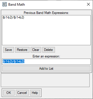
This seems reasonable……but if you do this,
you will end up with an image that consists entirely of 0 and 1 instead of the
decimal values we want. This is because you are starting with an image with a
Data type of “unsigned integer” and this will result in an output image with
the same data type and all decimal values will be rounded to 0 or 1.
Bummer.
So you need to learn
a new trick. You need to convert you unsigned integer values to floating point
values within the Band Math tool so your output image will have the floating point values we want. So you need to write an
expression like this: (float(b1)-float(b2))/(float(b1)+float(b2))
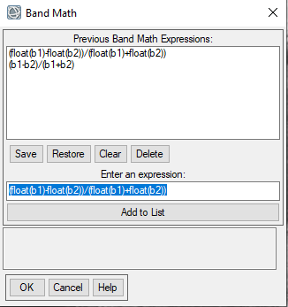
In the Variables to Bands Pairings
dialog box, be sure to select Band 8 for “b1” and Band 6 for “b2.” Run this
calculation for both the July 14 and the July 17 50 cm resolution images.
After doing this, and for each date, I
loaded both the 5 cm image and the 50 cm NDI image in ENVI. I viewed the 5 cm
image to enable me to precisely locate each panel, and
then toggled to the 50 cm NDI image and recorded the NDI value adjacent to the
panel. I’ve done this for you for all panels and all dates, including two other
dates that we will not use for this analysis.
The NDI values and the percent vegetation
coverage (including both eelgrass and algae) obtained from the virtual ground
truth panels is provided in the Excel file that is in the “eelgrass” folder.
Modeling Eelgrass Coverage: Open the Excel
file and take a look at these data. We will be using
regression analysis to use NDI to predict the percent coverage of eelgrass and
algae. You should be familiar with regression analysis from your statistics
course, but you can also google “regression analysis” to review. We will do
this regression analysis in Excel but if you are more comfortable using the “R”
stats package you can go this route.
In Excel, go to Insert-Charts and
select the scatter plot ![]() and just the version with a bunch of dots but
no connection of the dots. In the middle of your chart area, right-click and go
to Select Data. In the Select Data Source window, go to Legend
entries-Add. In the Edit Series window, give
your chart a Series name. Then in the Series X values click on the
little up arrow and drag over all of the NDI values.
Then for the Series Y values click on the little up arrow and select all of the “green stuff” values. Then click OK, the OK again
in the Select Data Source window. You should get something that looks
like this.
and just the version with a bunch of dots but
no connection of the dots. In the middle of your chart area, right-click and go
to Select Data. In the Select Data Source window, go to Legend
entries-Add. In the Edit Series window, give
your chart a Series name. Then in the Series X values click on the
little up arrow and drag over all of the NDI values.
Then for the Series Y values click on the little up arrow and select all of the “green stuff” values. Then click OK, the OK again
in the Select Data Source window. You should get something that looks
like this.
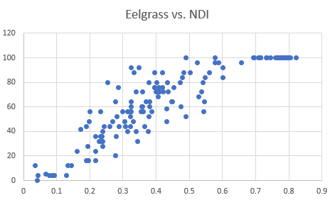
You can pretty this chart up by adding
axis labels.
This data looks pretty
darned good. There seems to be a strong relationship between the NDI
values and the percent coverage of eelgrass and algae. But we’d like to come up
with an equation to describe this relationship and we’d like to quantify the
strength of this relationship using an R-squared value. And what is an
R-squared value? Look it up.
To generate this equation in Excel, all
you need to do is right-click on the points and go to Add
trendline. This brings up the Format trendline dialog box. You can
choose between linear, logarithmic, polynomial or moving average. And down at
the bottom you should check the Display Equation on chart and
Display R-squared value on chart boxes. Try each of the trendline
options to see what gives you the best fit to your data. After deciding on the
best one, you should take a screenshot of the figure to include it in your lab
report. And, you will need the equation for the
next step!
Using your model: Back in ENVI, load
the July 14 NDI image that you generated from the 50 cm resolution image. Now
go to Band Math and use the equation that you generated in Excel to
create a percent vegetation cover layer. If you choose to use the equation with
the ln function, ENVI doesn’t understand “ln” when used in an equation. For
some reason, ENVI wants you to use “alog” instead. No
idea why.
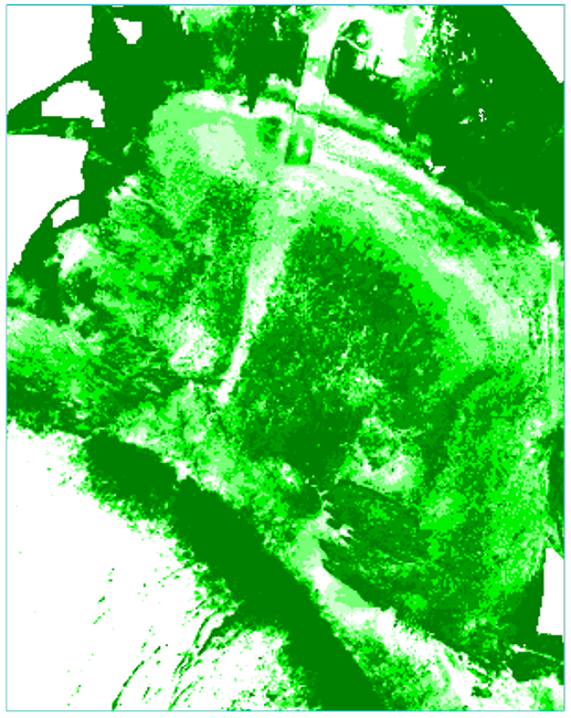
After using your equation to generate a
vegetation cover layer, you can create a raster color slice to define a few %
cover categories. I’d suggest perhaps 6 categories like:
<10%
10-20
20-40
40-60
60-80
80-100
For July 14, my result looks like this:
Do the same thing for your July 17 NDI
layer.
OK now we are really
only interested in the veg cover on the mudflat and the adjacent
subtidal areas. So, I’ve created a mask to enable you to eliminate all of the
upland from your veg cover layer. This is the “mud_clip” layer in the “eelgrass” folder. Open this layer
and take a look. You will note that all
of the upland has a value of 0 and the mudflat and adjacent subtidal
areas have a value of 1. You know this trick. Go into Band math and multiply
each of your vegetation cover layers by the mud_clip
layer. However, as you do so, you might want to convert your floating point vegetation cover values to signed integer
values. To do so in Band math, use this equation:
Int(b1*b2)
Fix(b1*b2)
(correction
added 3/5)
With your result as integer, rather than
float (decimal values) it is easy to go to Quick Stats and get the number of
pixels with each value. You can then export this to Excel and calculate the %
of the study area in each % cover category in your image.
After doing so, my July 14 veg cover layer
(with the same raster color slice applied) looks like this.
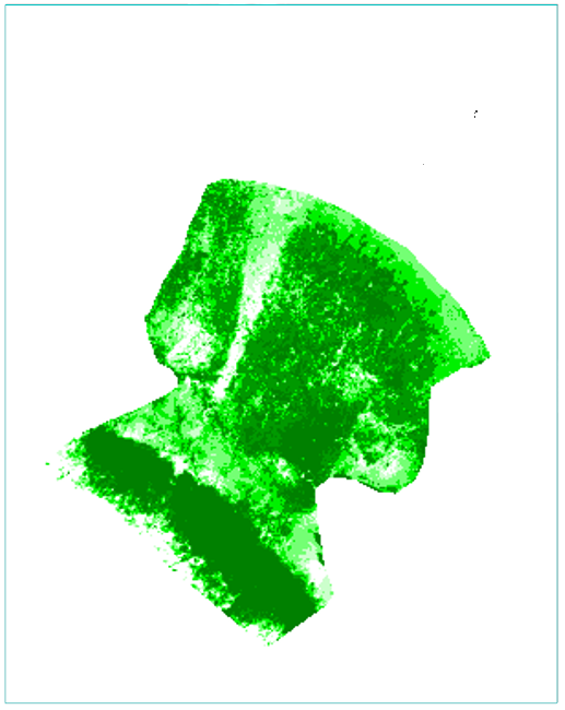
Do the same mud_clip
for the July 17 vegetation cover layer.
You can use the data from Quick stats
(exported to Excel) calculate the % of the mudflat in each of the % cover
categories in your figure.
Finally, we want to quantify the change
in vegetation cover between these two dates to see the impact of a busy weekend
(associated with the first weekend of recreational crabbing) at this boat ramp.
You know how to do this. Just use Band math and subtract the July 14 veg cover
layer from the July 17 veg cover layer (and used the versions clipped to just
the mudflat). Areas that lose veg cover will have negative values and areas
with an increase in veg cover will have positive values. I used these categories
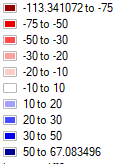
My result looked like this

As you can see, there was quite a bit of loss
of vegetation cover during this busy weekend.
That’s it: Prepare a lab
report for this exercise. In addition to the stuff above, you might want to use
quick stats to prepare tables showing the % of the mudflat that is in each of
the categories that you have illustrated in your figures.
Do I REALLY need to write another lab
report? Well,
maybe not. This is the sixth fifth lab (since we were not able to
complete Lab 6) exercise for which you could write a lab report. Your grade for
the lab portion of the class will be based on your best FOUR lab report
grades. So if you are happy with your grades so
far, you do not need to write a lab report for this exercise. But if you’d like
to try to bring up your lab report average grade a bit, this is a chance to do
so. It is entirely up to you.
As always, the report for this lab, if you
choose to write one, will be due on March 11, if you are in the TR lab or 12 if
you are in the WF lab..