Lab VI: Image Segmentation with SPRING

Objective: For today’s lab, we will conduct an image classification exercise using all 8 bands of the World View-2 satellite image. We will first conduct an image segmentation using a package called the Orfeo Toolbox, then classify the result using a k-means unsupervised classification routine in RStudio and finally assign the resulting spectral classes to information classes in ENVI. You will then evaluate the effectiveness of the analysis and to support your claims with qualitative and quantitative evidence from your results.

Preliminaries: In addition to using ENVI and Arc, you will also be using two other software packages that you will need to download onto your computer. To begin, go to the class files on Sharepoint site and grab both the “image_seg_downloads” folder as well as the “worldview2012” folders.

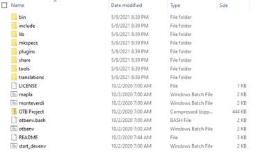
Load Monteverdi and the Orfeo Toolbox: We will begin by installing the software in the “image_seg_downloads” folder. One of the files in this folder is “OTB-7.2.0-Win64.zip”. This is a “zip file.” Zip files are compressed files that take up a fraction of the space of all of the files contained within it. Hopefully, you have a program called 7zip installed you your computer. Go ahead and launch 7zip and navigate to the “image_seg_downloads” folder and select “OTB-7.2.0-Win64.zip” and then click on Extract.” This will launch the unzipping process. You will be asked where to put all of the resulting files but the default will be to create a new folder with the name “OTB-7.2.0-Win64.” You can give it a different name or just take this default. After the unzip process finishes (which may take some time), you can go into this new folder. The contents should look like this:

Right-click on “Monteverdi” and create a shortcut to this file on your desktop. After doing so, double-click on Monteverdi on your desktop. If you have successfully loaded it, you should see this:

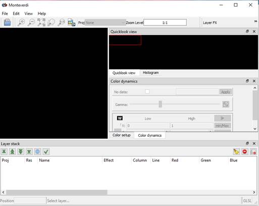
Monteverdi is an opensource GIS package that, among other things, includes the Orfeo toolbox that we will be using to do our image segmentation. We’ll come back to this below.

Note: If Monteverdi does not launch properly, try double clicking on the “maple.bat” file. This should bring up something that looks like this:

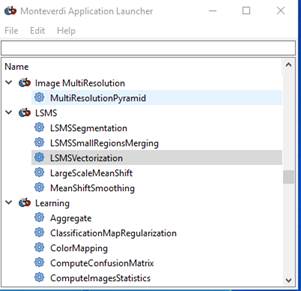
You may need to scroll down to find the LSMS functions that we’ll be using. Either interface will work for us. I’ll come back to this below.

Loading R and R Studio: This should be pretty simple. In the “image_seg_downloads” folder, double-click on “R-4.0.5-win.exe.” This should walk you through the process of loading R which is a very full-featured opensource statistics package. After this completes, double-click on “RStudio-1.4.1106.exe.” This should walk you through the process of loading RStudio which is a graphical user interface that you use to actually run the R software.

OK, you are now done with preliminaries and we can begin working with the imagery.

Introduction: For this lab, we want to use an image that was acquired by the World View-2 satellite. This satellite was launched in October of 2009 and the image that we are using was acquired on September 29, 2010. More information about this satellite is available HERE. Briefly, this satellite provides multispectral imagery with a spatial resolution of 2 meters for 8 bands.

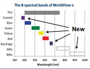
WorldView-2 is one of the “IKONOS-type” satellites that have been launched over the past decade. See my partial listing of similar sensors HERE. Unlike the other “IKONOS-type” satellites, WV-2 provides data in 8 rather than 4 bands. WV-2 includes 3 new bands in the visible part of the spectrum and 1 new band in the near-IR. As a very new sensor, very little work has been done to evaluate its performance in various applications. Here is a comparison of the 8 WV-2 bands with the Landsat TM/ETM sensor. The first 4 Landsat bands are nearly identical to the 4 bands on the other IKONOS-type satellites.

	WorldView-2			Landsat TM/ETM
	Band		Wavelength	Wavelength
	Name	Band #	Interval (um)	Interval (um)	Band #
Coastal		1	0.40-0.45
	Blue	2	0.45-0.51	0.45-0.52	1
	Green	3	0.51-0.58	0.52-0.60	2
	Yellow	4	0.585-0.625
	Red	5	0.63-0.69	0.63-0.69	3
	Red Edge	6	0.705-0.745
	NIR-1	7	0.77-0.785	0.76-0.904	4
	NIR-2	8	0.86-1.04
				1.55-1.75	5
				2.08-2.35	7

The image covers an area that is about 4 km by 4 km. This is a subset of a larger image:

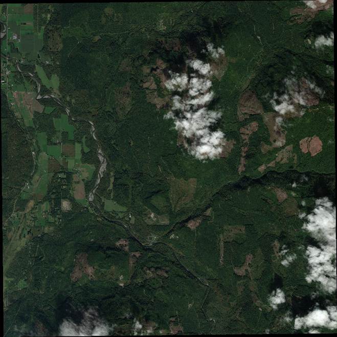
10SEP29191955-M3DS-052411962060_01_P001-BROWSE

Our image covers roughly the upper left quarter of this scene. In addition to the multispectral imagery, we also have a panchromatic image at ~0.5m resolution. This image covers the southern part of the valley of the South Fork of the Nooksack River. State Route 9 enters the scene in the NW corner of the scene and the small town of Acme is just south of where Rt. 9 crosses the S. Fork of the Nooksack.

Back to Outline

When using moderate resolution imagery (such as LANDSAT imagery with a pixel size of 30 m), pixel-based classification works quite well. Pixel-based classification involves classifying each pixel based solely on its spectral properties without considering the characteristics of any of the surrounding pixel. With high resolution (HR) imagery (pixel size of a few meters down to a few centimeters), pixel-based classification does not work. Instead, the emerging consensus is to perform image segmentation as a pre-processing step prior to classification. Image segmentation involve joining adjacent pixels with similar spectral properties into “image segments.” The image segments can be of irregular shape and size. Image segments are then classified on the basis of the mean and variance of the spectral properties of the pixels in each image segment. The spatial properties (shape and size) of each image segment can also be used as part of the classification process.

For today’s lab we will use a variety of software packages to carry out both the image segmentation and classification processes.

Back to Outline

PROCEEDURES

STEP 1: You should have already downloaded the worldview2012 folder from the sharepoint site. If not, see the link above and do so.

The image that we are using has the catchy name of: 10SEP29191955-M3DS_R1C1-052411962060_01_P001.TIFF

There are a few other files in this folder that you will need. Copy everything to your working directory under C:/temp

Back to Outline

STEP 2: Image Segmentation with Monteverdi and the Orfeo Toolbox:

This is an open source image processing package. I’m still on the steep end of the learning curve with this package but it seems to have some nice features. So here goes….

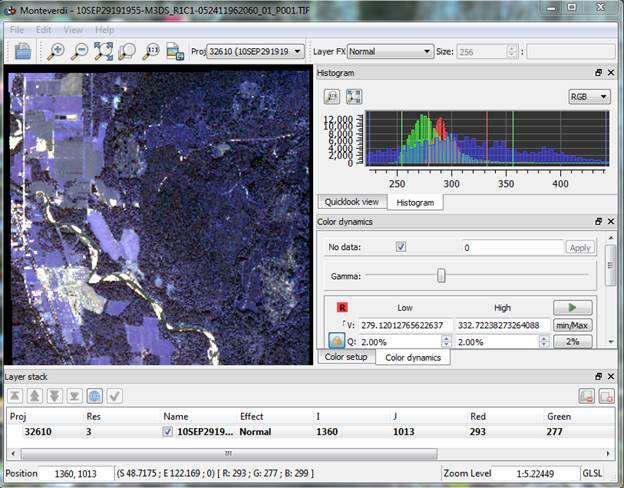
From the Monteverdi interface (if you were able to launch it) go to File-Open Images. Open your worldview image (10SEP29191955-M3DS_R1C1-052411962060_01_P001.TIFF). It should look something like this:

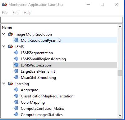
Monteverdi is an open source GIS and remote sensing package. I have not really begun to explore all of the features of this package. We are just going to focus on using it to perform the image segmentation process using a package called the Orfeo Toolbox (OTB). Open this package by going to View-OTB Application browser. This will add an OTB_Application browser new tab on the right side of your screen.

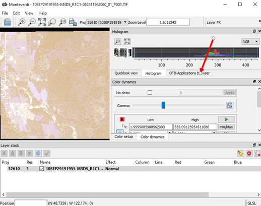
Click on this tab and enlarge the window for this tab, and it will look something like this:

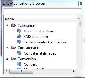
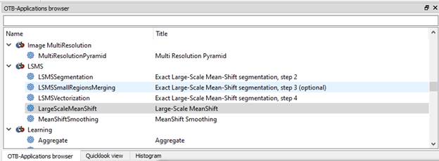
Or, if you could not get the full Monteverdi interface to open, you can get to the same stuff we need from this:

Grab the corner of this dialog box and enlarge it, then use the slider to find the Large-Scale Mean-Shift segmentation tools:

((insert link to papers about LSMS))

The LSMS process includes 4 steps. Here is a link with some documentation about the steps that we will be running: https://www.orfeo-toolbox.org/CookBook/recipes/improc.html#large-scale-mean-shift-lsms-segmentation

And here is a link to the paper that is referenced above Michel_et_al_2015_Stable_Mean_Shift_algorithm

And here is another paper that I found to be quite useful:

Chehata_etal_2014_Object-based change detection using high-resolution multispectral images.pdf

Back to Outline

The Mean-Shift Segmentation Algorithm:

Briefly, the MSS algorithm works by searching for local modes in the joint feature (spectral) and spatial domains. In geek-speak, the algorithm “searches for local modes in the joint feature and spatial domain of n+2 dimensions, where n is the number of features (spectral bands) that are added to the two spatial dimensions.” So, just like ISODATA, LSMS is identifying pixels that are close together in spectral space but ALSO close together in geographic space; the spatial dimensions. There are two parameters that control the segmentation process. The spatial radius controls distance (number of pixels) that is considered when grouping pixels into image segments. The range radius refers to the degree of spectral variability (distance in the n-dimensions of spectral space) that will be permitted in a given image segment. The range radius should be higher than the maximum spectral difference between intra-segment pixel pairs and lower than the spectral difference between segment pixels and the surrounding pixels outside the segment. The spatial radius should be close to the size of the objects of interest (Chehata et al. 2014).

I’ve done a whole bunch of segmentations with a different image (centimeter resolution image acquired from an unmanned aircraft) using a range of parameters. Just to give you a feel for the different results, here are some examples using different combinations of spatial radius and range radius. In each of the four examples below, I used a minimum region size of 500 pixels (about 0.5 m^2).

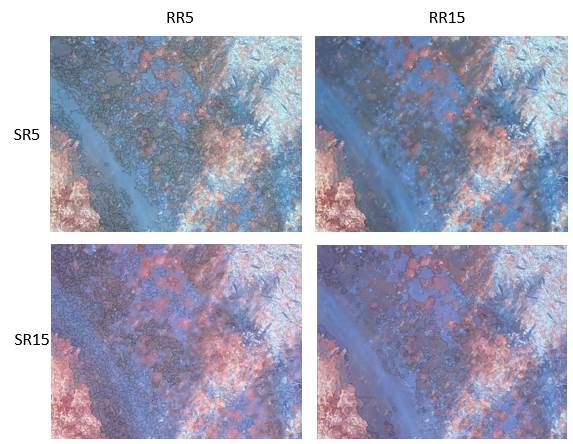
Note that as the SR and RR increase, the resulting image segments get larger and seem to include scene components that are obviously quite different (eg, vegetation and rock). After experimenting quite a bit, I found that I was not able to obtain “clean” image segments until getting down to SR: 2 and RR: 4.

Parameter selection in this segmentation step is critical. If the segments are too large, dissimilar objects are included within each segment and within-segment variability compromises the classification accuracy. If the segments are too small, individual objects in the scene (e.g. a single building or a single tree canopy) will be subdivided into separate image segments and the spatial properties of these objects will be lost. Methods for optimizing parameter selection are under development in the literature. At present, parameter selection is mostly done using trial and error. Here is one paper that presents a possible approach to optimize parameter selection. (Ming_etal_2015).

For today’s lab I’ve just taken a wild guess at parameter selection. We will perform a segmentation (the 4 steps outlined below) using ~~SR: 9, RR: 70 and a minimum segment size of 40.~~

~~NOTE added 2/21/2018: Or you can try these parameters; SR: 23, RR: 285, M:132. Not sure if this will produce a better result. Definitely results in fewer image segments.~~

~~NOTE added 2/17/2020: Or you can try these parameters; SR: 23, RR: 285, M:132. Not sure if this will produce a better result. Definitely results in fewer image segments.~~

NOTE: 5/9/2021: Let’s use SR: 23, RR: 61, M:132

Back to Outline

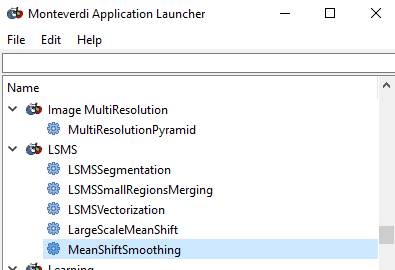
The last option, the “MeanShiftSmooting” is Step 1. You should start with this. The “LargeScaleMeanShift” option (2^nd from bottom) is new and, based on reading the documentation, it appears that selecting this allows you to run all 4 steps at once. I’ve not tried this so not sure that it is exactly equivalent (does it run the “optional” 3^rd step?), so I’d suggest you run the 4 steps one at a time. And, due to the version updates, the dialog boxes may be a bit different.

Run LSMS Step 1: Large-Scale Mean-Shift (LSMS)

Let’s start with Step 1. Read the documentation (link above), then specify your input image and filenames for the “Filtered output” and the “Spatial Image.” (be sure to give each of these output files a .tif suffix) I’d strongly recommend that you put all of your output files in a separate folder. I called mine “segout.”

Input image: this is your worldview image; 10SEP29191955-M3DS_R1C1-052411962060_01_P001.TIFF

I’m putting all of my output in my “segout” folder which I’ve created inside my worldview2012 folder

Filtered output: I used a filename of; acme_s23_r61_spectral_filtered_step1.tif

Spatial output: I used a filename of; acme_s23_r61_spatial_filtered_step1.tif

Input your spatial and range radius, then take all of the other default parameters EXCEPT, you should make sure that the Mode Search option is OFF. Mine looks like this:

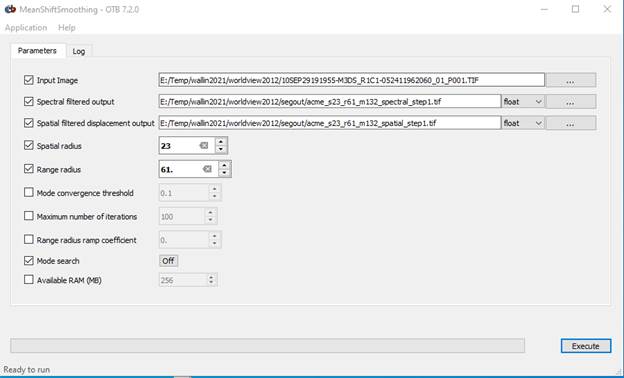
Then hit the Execute button.

NOTE ADDED 2/17/2020: Many of my screenshots below show S23, R92, M40. Ignore and go with S23, R61, M132

As it is running, the green “Ready to run” text will change to red “Running.” A progress bar move as processing proceeds. The red “Running” message will change back to the green “Ready to run” text when processing is complete.

Back to Outline

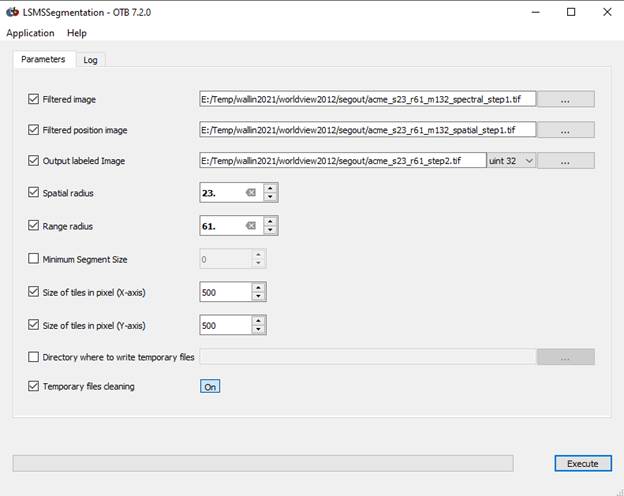
Run LSMS Step 2: LSMS Segmentation

The labels in the Step 2 dialog box are not clear. Your output files from Step 1 will be used here. In the Step 2 dialog box, for the “Filtered image” use the use the “Spectral Filtered” output image from Step 1. For the “Filtered position image” use the “Spatial filtered” output image from Step 1.

Specify an output image (with a .tif suffix). I used a filename of “acme_s23_r61_step2.tif.”

Input your spatial and range radius values again. Don’t set a Min Region Size. If you set a Min Region size here, these small regions will be set to the background label and will not be subject to further processing. This would lead to “holes” in your final output. We’ll deal with these small regions in a different way in the next step.

Click Execute but be patient. It appears that nothing is happening, but all is well. Unlike with Step 1, there is no progress bar. Unlike Step 1, Step 2 runs pretty quickly.

When this step finishes, your acme_s23_r61_step2.tif will be displayed (if you have the full Monteverdi interface that displayed the original image). Mine looks like this:

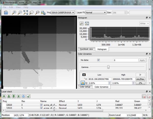
The blocky nature of this image is just an artifact of the way that the image segments are labeled at this point and the fact that the segmentation proceeds in “tiles” or subsets of the full image. This means that each of the segments in a given tile are labeled sequentially. The labeling starts with the image segments in the upper left tile (low label numbers; darker shading) and the labels for the segments in the lower right get higher label numbers and hence lighter shading. This issue will be addressed in later steps.

Back to Outline

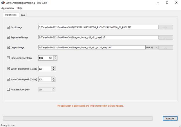
Run LSMS Step 3: LSMSSmall Regions Merging Application

This step can be used to filter out small segments. Segments below the threshold size are merged with the closest big enough adjacent region based on radiometry.

The “Input image” is your original worldview image. The “segmented image” is the output from step 2. Specify an output image with a .tif suffix. I used “acme_s23_r61_m132_step3.tif.”

Let’s go with a Minimum Region Size of 132. With 2 m by 2 m pixels, a region composed of 132 pixels would have an area of 132*2*2 = 528 m^2.

Click Execute and again be patient. It is not clear that processing is underway but it is.

Back to Outline

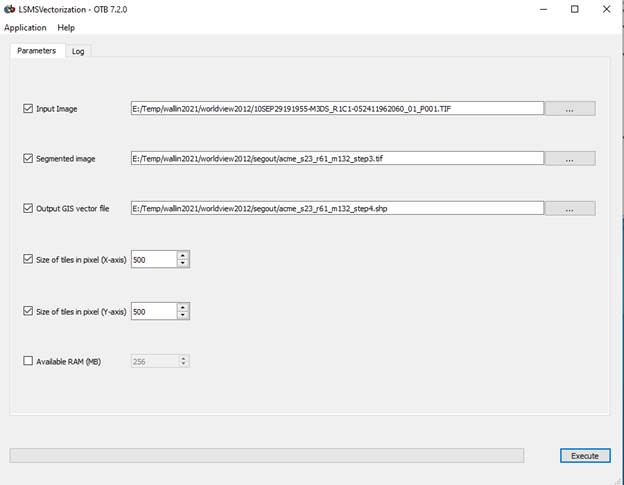
Run LSMS Step 4: LSMSS Vectorization

This step produces a vector output of the segmented image. The output is a shapefile that with a polygon that delineates each image segment. For each image segment, the attributed file provides the mean and variance of the brightness value for each band for all pixels in the segment and the number of pixels in each segment.

Again, the “Input image” is your original worldview image. The “Segmented Image” is the output from step 3. The output file is a vector file and it must have a .shp suffix. I used an output filename of “acme_s23_r61_m132_step4.shp.”

Again, click Execute and be patient.

Back to Outline

STEP 3: Examine your Image Segmentation Result in Arc

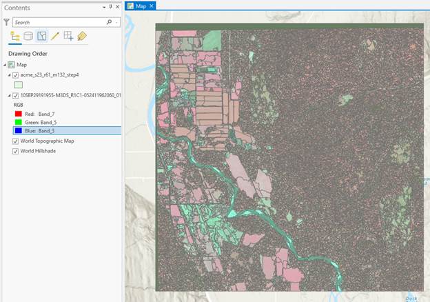
Open ArcPro. Create a new project, then go to the Map tab and the Add Data button

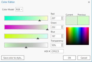
to add both your original Worldview image and the shapefile that you created in Step 4 in OTB (mine is called “acme_s23_r61_m132_step4.shp.”). Turn both on. If you have the shapefile on top, you can right-click on the color box (below the shapefile name in the Contents panel) go to Color Properties and in the Color Editor window, set the Transparency to 50%.

and go to Properties-Display and set the transparency to 50% so you can “see through” the shapefile to see the image below. Mine looks like this:

From the Contents, right-click on your shapefile and Open the Attribute Table. The first part of mine looks like this.

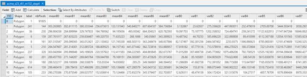
Each row in the table represents one image segment. So note that in my case, my segmentation consists of ~13000 image segments. The fields in this table are:

FID: is just a segment ID#.

Shape: all are polygons

Label: I have no idea what this is??

nbPixels: the # of pixels in the image segment

meanB0,.., B7: mean value in band 0 through band 7 (no idea why they don’t number them 1-8 but it doesn’t really matter) for all of the pixels in a given image segment

varB0,.., B7: variance of the values in B0,..,B7 for all of the pixels in a given image segment

All of the information in your attribute table is saved in a .dbf file with the same prefix as your shapefile. Open the .dbf file in Excel and save a copy as an Excel file. For some reason, the FID does not get saved as part of the dbf file. So in the Excel file, you will need to insert a column, label it “ID” and insert segment id# starting with 0. Also, very important, delete the “Label” column!!!!!

We now want to carry out an image classification.

But first, we will convert all of our variables (nbpixels, meanB0…B7, varB0…B7) from their raw values to Z-scores. This is easy to do in Excel. For each variable, calculate the average and the standard deviation. Then, on a separate worksheet, calculate Z-scores using this formula:

Zscore = (X – average)/standard deviation

I’ll demonstrate how to do this in lab.

The classification will be done using the Z-scores for all 17 variables (nbpixels, meanB0…B7, varB0…B7). If you would like, you could also experiment by doing the classification using subsets of these variables (means only, means and variance only).

After calculating Z-scores for all 17 variables, Thesave this new worksheet (with just the ID and all 17 variables) as a “Comma Separated Variable” file (.csv file format). This reads into R most easily.

Before bringing this file into R, you should open your file using Notepad and check to be sure that there ARE NOT a bunch of extra commas at the end of each line. If there are, you will not be able to read this file in R.

We will be doing the unsupervised classification in R Studio.

Back to Outline

STEP 4: Image classification in R:

Open R Studio. At this point, we want to perform an unsupervised classification using a routine called K-means. This routine will identify image segments that have similar spectral (mean in B0,….B3) properties as well as within-segment variance for each band as well as segment size (number of pixels in each segment). Image segments with similar properties will be assigned the same group. We will refer to these groups as Spectral classes and each will have a unique spectral class ID number. At a later step we will then assign these spectral classes to Information classes which will be things like vegetation, rock, logs, water.

After opening RStudio, go to File-New File-R Script. This will open a new window in the upper left portion of the RStudio app.

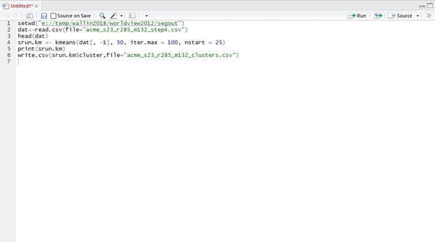
Just copy and paste this entire script below into the window you just opened (upper left window in R Studio). Note that the text in green that follows the # are just notes describing what each section does the text in red indicates things that need to be changed depending of your folder and filenames:

#next line sets your working directory change to where ever you are working

setwd("c://temp/wallin/worldview2012/segout")

#Note that you will need to change the filename and sheetname below if yours are different

#And Note that you will have to change the endRow below if you had a different number of #segments in your file

dat <- read.csv(file="acme_s23_r61_m132_step4.csv")

#next line just prints out the first few rows of the file just to confirm that it was properly read in

head(dat)

#this runs the kmeans routine on our data using everything except the ID as predictor variables

#it will produce 50 spectral classes, run 100 iterations and use 25 random starting points

#the output goes to an output data matrix called srun.km

srun.km <- kmeans(dat[, -1], 50, iter.max = 100, nstart = 25)

#next line displays a bunch of output

print(srun.km)

#writes an excel file (use a different name if you prefer) containing a single columns of numbers

#representing the predicted spectral class number

write.csv(srun.km$cluster,file="acme_s23_r61_m132_clusters.csv")

After pasting all of this into RStudio, it should look like this:

Now highlight this entire script and hit the button at the top of the Console window.

It should chug for a bit then spit out some output. Mostly, you want to make sure that it has created the “acme_s23_r61_m132_clusters.csv” file (or whatever you chose to name it. When you open this file, you will note that it has the spectral class assignments for all ~13000 image segments. Note that it just contains a single column of numbers with a column header of “x” and an unnamed column starting with “1” to designate the segment numbers. You should label this column with something like “ID”. Then renumber the rows starting with the number zero. The easiest way to do this is with the Fill-Series function:

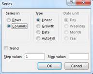
The stop value should be ~13059 (or however many image segments you ended up with; it will be different if you used different parameters when doing the segmentation). Scroll to the bottom of the file to confirm that you have done this properly. After doing this, save this as an Excel file.

At this point, you are done with RStudio

Back to Outline

STEP 5: Back in Arc…. Join Data and Create Raster

Back in Arc, right-click on your shapefile and Open the Attribute Table again. For each image segment in the attribute table, we now want to add the spectral class ID number that we just generated in R using the K-Means unsupervised classification routine.

In the Table of Contents window, Right-click on your segmentation output shapefile (mine is “acme_s23_r61_m132_step4”) and open the Attribute table.

Join data:

In the attribute table window, click on the on the top right side of this window. Table option button and go to Joins and Relates-Add Join. In the Add Join dialog box,

Your “Input Table” is your shape file. The “Input Join Field” is the FID from the shapefile.

You also need to go back to the Add data button and add the CSV file that contains your clusters (the product of doing the classification in R).

The “Join Table” is your CSV file with the clusters and the “Join Table Field” is the ID label that you added to the clusters. The dialog box should look like this:

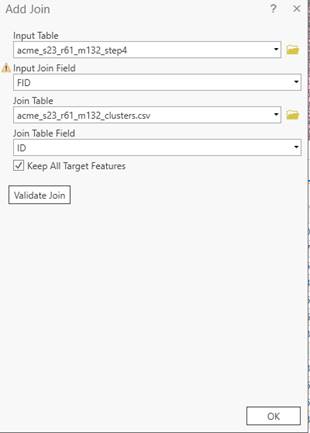
Click OK. Arc will chug for quite awhile as it complete the link for all of the ~13000+ image segments. When it finishes, you will see two more columns added on the right side of your attribute table, “ID” and “x”.Note that you just created a dynamic link between your Attribute Table and the Excel file.

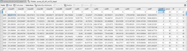
Here is one way to add these columns to the attribute table on a permanent basis. In the upper left corner of the window displaying the attribute table, click on “Add” This adds a new field to your attribute table. Give it a name. something like “JoinID” might be good. Just below, click on this to add one more field. Name it something like

“JoinCl.” Then go back to your attribute table and slide over to the right. You should now see the two new columns you added along with the two columns from the dynamic join.

You now want to copy the values from the dynamic join into your two new columns. To do so, right-click on “joinID” and go to Calculate Field. In the Calculate Fields dialog and the Fields section of this dialog, scroll down and double-click on “ID” (recall that this is the field added by the dynamic join that is identical the “FID” in your original attribute table). Complete this process by hitting Apply and then OK.

Repeat this process to copy the values from the “x” field (these are the cluster values from the dynamic join) into your new “JoinCl” field. After doing so, the upper part of your attribute table should look like this:

Create a new raster file:

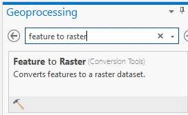
At this point, we want to create a new raster file with the same cell size as the original starting image (the Worldview image) but with every pixel having the spectral class number (the cluster values) that we just added to the Attribute Table above. To do this, go to the Analysis tab in the ribbon at the top and go to Tools. In the Geoprocessing window, search for Feature to raster.

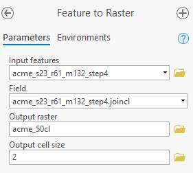
Select this and enter the proper parameters:

Input feature: is the shapefile that you have been working with

Field: the column in the attribute table containing the spectral class numbers (in my case JoinCL)

Output raster: select a folder and new name for the output file

Output cell size: very important! Change this to “2”. A 2 meter cells size; same as your original worldview image.

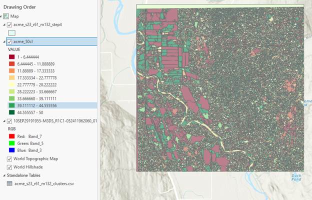
Then hit Run. Arc will chug for a bit, then add this new raster to your Table of Contents. Take a look at it. You might need to right-click on your output raster and go to Properties-Symbology-Unique Values to get each segment to display with a unique value. I’ve done all of these steps for a bunch of different parameter values.

Mine looks like this for s23_r61_m132:

Export to ENVI:

Next we need to move back to ENVI to assign spectral classes to information classes. Before we do, we need to export your new raster to a format that ENVI can read. Right-click on your new raster and go to Data-Export Raster. In the Export Raster dialog, select a Location and a Name. It is also very important to select a Format which you should set to ENVI. Then Export.

Back to Outline

STEP 6: Assign Spectral Classes to Information Classes: When you first bring your file into ENVI, it will come in as an ENVI Standard file, but you need to convert it to an ENVI Classification so you can edit the Class names and colors. To do so,

- open image in ENVI

- go to View Metadata->Edit Metadata

- select the add metadata (+) from the top of the dialog

- select attributes 'number of classes', 'class colors', and 'class names' - items are added to the bottom of the dialog

- set number of classes; default class colors and names are added - alter as needed

- save the metadata by selecting 'ok' in the dialog.

The file should close then automatically reopen and display as a 'classified' image.

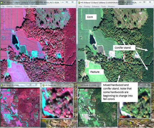
You know what to do from here. Open your classified image in ENVI. At the same time open the raw TIFF in two different displays; one as a color-IR image (bands 7, 5, 3 into the RGB layers, respectively) and also as a “true color” display (bands 5, 3, 2 in the RGB layers, respectively). Link all three displays to confirm that everything lines up properly. You may need to play around with the enhancements to improve the appearance of these images, especially the color-IR image (I found that a square root enhancement on the scroll window looked pretty good). Move around the images a bit to get familiar with the area.

Recall that the image was acquired in late September. In the true color display, you will note that some of the trees are changing color. These are deciduous trees (mostly red alder, bigleaf maple and cottonwood).

Do your best to assign the spectral classes in each classification to one of the information classes listed below. You should also add a “shadow” class.

Just to get you started, here is a detail of part of the image:

Young conifer stand; ~15 years old.

~50 year old conifer stand. Some understory deciduous understory vegetation may be visible through canopy gaps.

Do your best to assign the spectral classes to information classes based on visual cues in the images plus your experience with previous labs. We have a very limited set of ground data and I want to save that for an accuracy assessment. We will discuss the image in lab and point out a few more visual cues that can be used. Try to assign your spectral classes to the following information classes

Code	Description
111	Residential
120	Farm Building
141	Road
172	Shrubs
211	Crops
212	Pasture
400	"Recent" Clearcut
410	Deciduous forest
420	Conifer forest
510	Water
20	Nonforested Wetland
740	Rock/Gravel bar/soil

After assigning each of your 50 spectral classes to these 12 classes (and you should try to assign at least one spectral class to each of these 12 classes), you should run a combined classes step create a 12 class map (maybe 13 if you added a shadow class).

Back to Outline

Step 7: Accuracy Assessment: The folder for this lab (J:\saldata\Esci442\worldview2012) includes an excel file (pcq_lulc_data_acme.xls) with ground truth data. We have ~150 points with LULC Level3 codes that can be used to conduct an accuracy assessment. We also have ~40 PCQ points and we will use these data for a LIDAR lab in a few weeks. Using the data in the Excel file, I have created an ROI file for you to use (test12_2017.roi). This file includes points for each of the 12 information classes listed above.

NOTE Added 2/22/19: I just discovered that there is something weird with the test12pts_2017.roi file. When you open this file, it will appear with 31 classes, most of which seem to be left over from our BakerBay Unsupervised classification. In File-Data Manager, this roi looks like this:

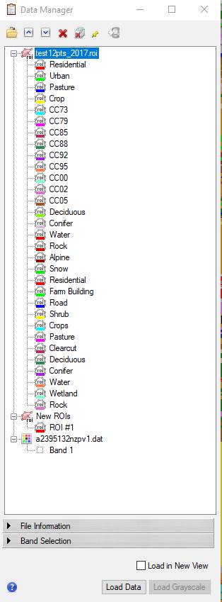
Most of the classes in this ROI are left over from the previous unsupervised classification. Not sure how this happened. Here is a work around. Bottom line is that you want to delete the unwanted classes. To do this,

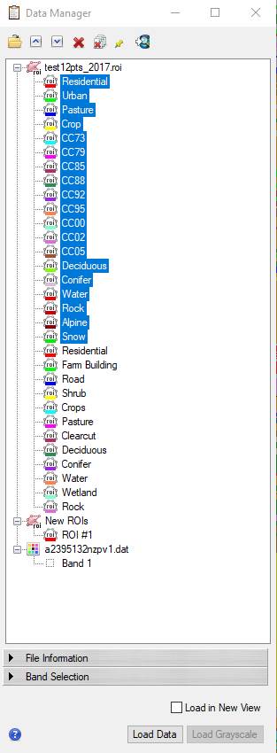
-click on the “Residential” class at the top of the list to highlight it,

-then hold down the shift key and click on the “Snow” class resulting in this:

-Then click on the red X button at the top of the dialog box, resulting in:

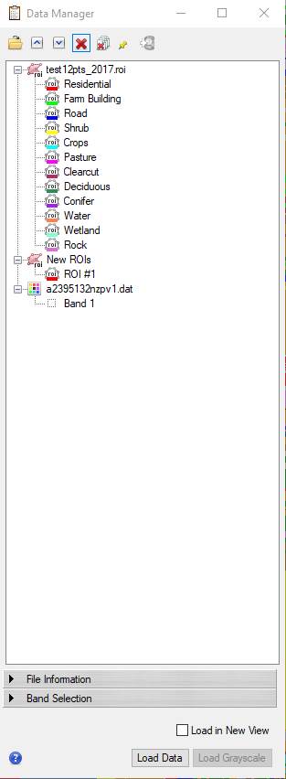
-Then proceed with generating the confusion matrix as you did in the Baker Bay Unsupervised classification exercise.

You should generate a confusion matrix using this ROI file. Finally you can drop your results into my “class_acc.xlsx” file to see how your classification accuracy changes as some of these classes are combined.

And yes, you will be writing a lab report for this exercise.

Return to ESCI 442/542 Lab Page

Return to ESCI 442/542 Syllabus

Return to David Wallin's Home Page