Lab VI: Image Segmentation with SPRING

Objective: For today’s lab, we will compare results obtained using all 8 bands of the World View-2 satellite to the results obtained when restricting the analysis to only the 4 bands that are available on the other IKONOS-type sensors. Your secondary objective will be to evaluate the effectiveness of the analysis and to support your claims with qualitative and quantitative evidence from your results.

Introduction: For this lab, we want to use a new image that was acquired by the new World View-2 satellite. This satellite was launched in October of 2009 and the image that we are using was acquired on September 29, 2010. More information about this satellite is available HERE. Briefly, this satellite provides multispectral imagery with a spatial resolution of 2 meters for 8 bands.

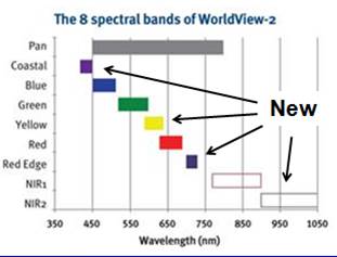
WorldView-2 is one of the “IKONOS-type” satellites that have been launched over the past decade. See my partial listing of similar sensors HERE. Unlike the other “IKONOS-type” satellites, WV-2 provides data in 8 rather than 4 bands. WV-2 includes 3 new bands in the visible part of the spectrum and 1 new band in the near-IR. As a very new sensor, very little work has been done to evaluate its performance in various applications. Here is a comparison of the 8 WV-2 bands with the Landsat TM/ETM sensor. The first 4 Landsat bands are nearly identical to the 4 bands on the other IKONOS-type satellites.

	WorldView-2			Landsat TM/ETM
	Band		Wavelength	Wavelength
	Name	Band #	Interval (um)	Interval (um)	Band #
Coastal		1	0.40-0.45
	Blue	2	0.45-0.51	0.45-0.52	1
	Green	3	0.51-0.58	0.52-0.60	2
	Yellow	4	0.585-0.625
	Red	5	0.63-0.69	0.63-0.69	3
	Red Edge	6	0.705-0.745
	NIR-1	7	0.77-0.785	0.76-0.904	4
	NIR-2	8	0.86-1.04
				1.55-1.75	5
				2.08-2.35	7

Back to Outline

Starting with a TIFF file, you will bring the image into SPRING and performed two image segmentations; one using all 8 bands and the other using only the 4 bands present in other IKONOS-type sensors. You will start by using a minimum mapping unit size for both segmentations of 25 pixels. With a pixel size of 2 m by 2 m, this translates to an area of 100 m^2, which roughly approximates the zone of influence for a single canopy dominant tree. You will then perform an ISODATA unsupervised classification on each segmentation, first using all 8 bands and then again using just 4 bands. You will then save the results as TIFFs, import these TIFFs into Arc, save them as an ENVI standard file, then bring them into ENVI and convert them to an ENVI classification file.

The image covers an area that is about 4 km by 4 km. This is a subset of a larger image:

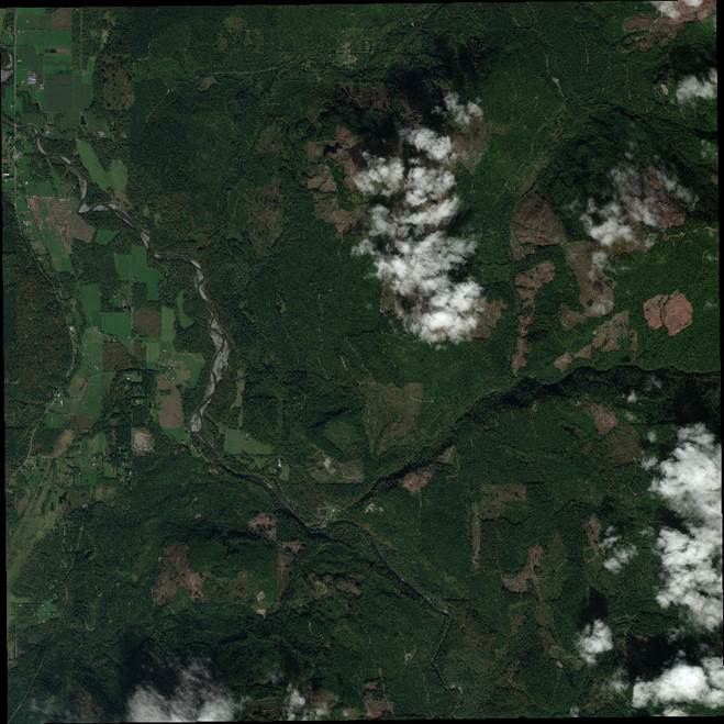
10SEP29191955-M3DS-052411962060_01_P001-BROWSE

Our image covers roughly the upper left quarter of this scene. In addition to the multispectral imagery, we also have a panchromatic image at ~0.5m resolution. This image covers the southern part of the valley of the South Fork of the Nooksack River. State Route 9 enters the scene in the NW corner of the scene and the small town of Acme is just south of where Rt. 9 crosses the S. Fork of the Nooksack.

Back to Outline

PROCEEDURES

STEP 1: Get the Data, Grab the entire folder named: J:\saldata\Esci442\worldview2012

The image that we are using has the catchy name of: 10SEP29191955-M3DS_R1C1-052411962060_01_P001.TIFF

There are a few other files in this folder that you will need. Copy everything to your working directory under C:/temp

Back to Outline

Step 2: Use IMPIMA to import your TIFF file and create a .spg . SPRING actually consists of a set of three programs:

SPRING – the image processing and GIS package;

IMPIMA – for image import and export;

SCARTA – for generating and printing maps (we will not be using this package).

We need to begin by using IMPIMA to bring our TIFF file into a format called GRIB that is used by SPRING.

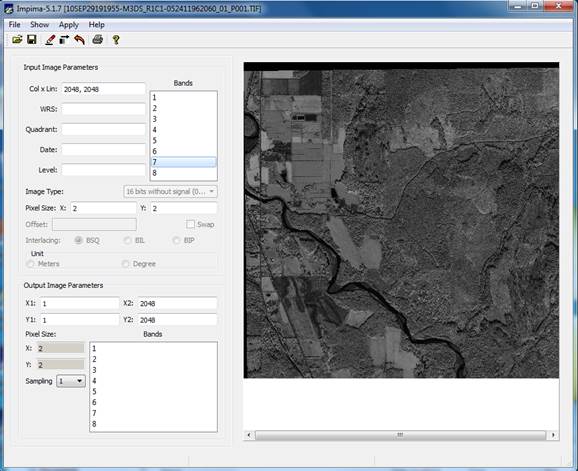
Begin by starting the IMPIMA-5.2.6 software. (NOTE: some of the screenshots below may be for the older 5.1.7 version) From the main toolbar, go to File-Open and select your TIFF file. Assorted file parameters will now be visible in the Input Image Parameters section including:

Col x Lin: 2048, 2048 (this is the number of columns and lines in the file)

Pixel Size X: 2.00 Y: 2.00 (this is the pixel size: 2m by 2m)

Note that the Image Type is 16 bit.

Highlight Band 7 (this is NIR-1) in the Input Image Parameters section and then go to Apply(Execute)-Draw or push .

In the Output Image Parameters section, click on all 8 bands and change the Sampling to 1. This will retain the same 2m by 2m pixel size in the output image. Now go to File-Save As or push and select a destination and output filename. I’d suggest a simple, descriptive name like “acme.” Two output files will be created; one small file with a *.dsc extension and another much large file (about the same size as your *.tiff file) with a *.spg extension. ~~Note that it will take some time to create these output files. In my case, with a *.tiff file of about 32 Mbytes, it took about 15 minutes to create the output files~~.(This actually seemed to go very fast; maybe an improvement in v5.1.8 of the software?) While these files are being created, the programs provides no feedback to indicate progress and the task manager indicates that IMPIMA is “not responding.” It will take a minute, maybe two. Be patient!

After your output files are generated, go to File-exit to close IMPIMA.

Back to Outline

Step 3: Open your file in SPRING. Start the SPRING-5.2.6 software. After closing the “News” panel, the initial window looks like this:

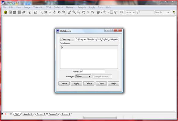
Create a SPRING Database: We need to begin by creating something called a SPRING Database. My working folder for this lab is c:/temp/wallin15/worldview2012. I have placed my the tiff file, acme.spg and acme.dsc files in this folder. Under worldview, (and using “My Computer”) I have created another folder which I called springdb. This is where my SPRING database will reside. From the Databases dialog box (NOTE: if the Databases dialog box does not appear when you start Spring, go to File-Database to bring it up), Click on Directory and navigate to the springdb folder (mine is c:/temp/wallin2016/worldview2012/springdb). Enter a name for your database (I used “acme_db”) and select the database type (this is called the “Manager” for some reason) as ~~“Access”~~ “SQLite”

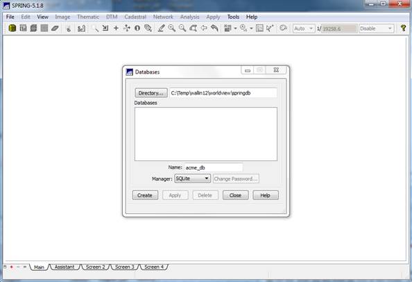
Click Create. If asked whether you want this database to have a password, select No. After your newly created database appears in the “databases” list, click on Apply in the Databases dialog box. The dialog box will disappear.

Back to Outline

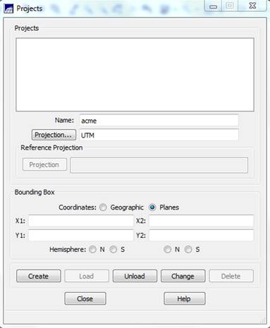
Create a SPRING Project: The SPRING Project defines the projection and bounding box (location and spatial extent) of your image. From the main SPRING toolbar, go to File-Project-Project. From the Projects dialog box, enter a Name (perhaps, “acme”), then click on the Projection button.

In the Projections dialog box enter:

Systems: UTM

Earth Models: ITRF(WGS84) (not certain of this, NAD83 might be OK as well).

NOTE: If use an image that is in NAD27, use Elipsoid->Clarke-1866

Note that the Hemisphere is selected as “South” and that this can’t be changed (bias in the software given that it was created in Brazil?). This may create problems later.

Origin

Zone: 10 (note that as soon as this is entered, the “Long” below fills in as:

Long: o 123 0 0.00

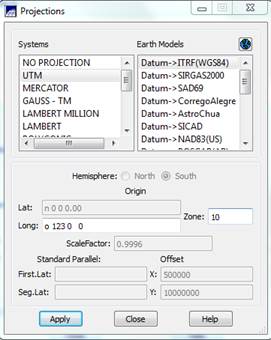
then Apply and the Projections dialog box will disappear.

Back in the Projects dialog box, set the Coordinates checkbox to Planes (to enable us to use UTM coordinate rather than latitude/longitude) and enter the coordinates of the lower left (x1, y1) and upper right (x2, y2) of your image. These can be obtained in ENVI by opening your starting tiff file

(10SEP29191955-M3DS_R1C1-052411962060_01_P001.TIFF). In the Available Bands List dialog, right-click on the image and go to Edit Header. In the Header Info dialog box, note the number of samples (e.g. columns) and lines (e.g. rows) in the image. Now go to Edit Attributes-Map Info. Under Map Coordinate of Tie Point you can obtain the UTM coordinates of the CENTER of the pixel in upper UPPER LEFT corner of the image.

Unfortunately, SPRING needs the coordinates of the LOWER LEFT AND UPPER RIGHT! Like this:

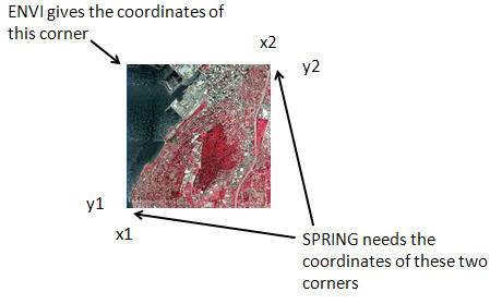
Although it is not entirely clear to me, I think that the coordinate given by ENVI above represents the CENTER of the pixel in the upper left corner of the image. Similarly, although it is not clear, I think that SPRING also needs the coordinates of the CENTER of the pixels in the lower left and upper right corners.

For the WorldView-2 scene of Acme (R1C1 from my data), here is the header info from ENVI:

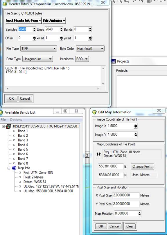
Note that the coordinates for the UL pixel are different in the Available Bands List vs. the Edit Map Information dialog. I suspect that the coordinate in the EMI window is for the center of the 2 m pixel and the coordinate in the ABL is for the upper left corner of the pixel but not sure. Still not sure if Spring wants the coordinates for the center or corner of the pixel. I will assume that SPRING wants the center of the pixel. So:

X1 = 558380 +1 = 558381

Y1 = 5398410 – (2048*2) -1 = 5394313

X2 = 558380 + (2048*2) – 1 = 562475

Y2 = 5398410 -1 = 5398409

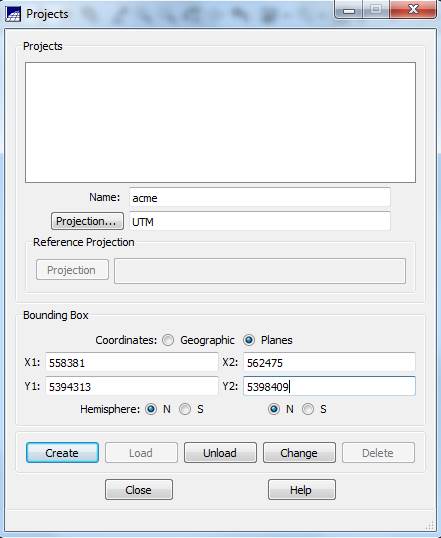
Select the Northern Hemisphere (BOTH PLACES!!!). Then click on Create, then Load.

Back to Outline

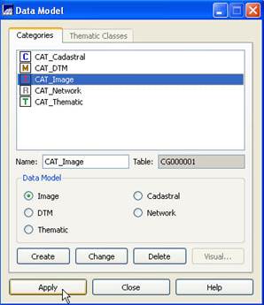
Create a Data Model: From the main SPRING toolbar, select File-Data Model. From the Data Model dialog box, under Categories select the CAT_Image. Then click on Apply (Execute in 5.1.8) and Close. It will appear as if nothing has happened. Trust me, all is well.

Back to Outline

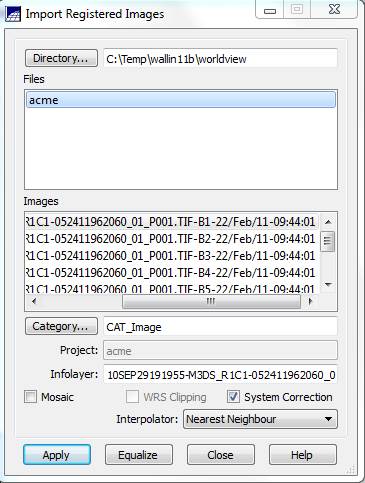
Import the image (finally!): From the main SPRING toolbar, select File-Import-Import Registrated (sic) Image. This brings up the Import Registered Images dialog box. Initially, you will probably get a warning indicating that:

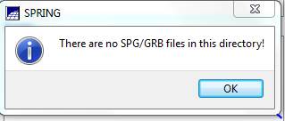
Click OK and then Click on the Directory button and navigate to the folder containing your .spg file (the .spg file was created from the .tiff file in IMPIMA). Your .spg file will show up in the Files window and the individual bands will show up in the Images window. It is not entirely clear to me but it appears that the layers in the Images window come from the .tiff file rather than from the .spg file. At any rate, click on the first band (10SEP29191955-M3DS_R1C1-052411962060_01_P001.TIF-B1-22/Feb/11-09:44:01 in my case) and, next to the Category button, make sure that it is set to CAT_Image. 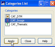If it isn’t click on the Category button to bring up the Category List dialog box. Select CAT_Image, and Apply

Back in the Import Registered Images dialog box, click on the System Correction box, leave the Interpolator set to “Nearest Neighbor,” then click on Apply.

A box will pop up informing you that you have an “Image without control points!” Click OK to dismiss this window. Another window may pop up informing you that you have an “Invalid threshold.” Click OK to dismiss this window. I have no idea what these messages really mean. At any rate, at this point, your first band should now appear in the Available Infolayers window of the Control Panel.

Back in the Import Registered Images dialog box, repeat this process for your other bands. Move the scroll bar along the bottom of the “Images” portion of the window to the right in order to view each band’s number (B1-B8). After doing this for all 8 bands, go ahead and Close the Import Registered Images dialog box. Verify that your correctly imported each band by moving the scroll bar in SPRING’s Available Inforlayers window to the right to again view each band’s number.

Back to Outline

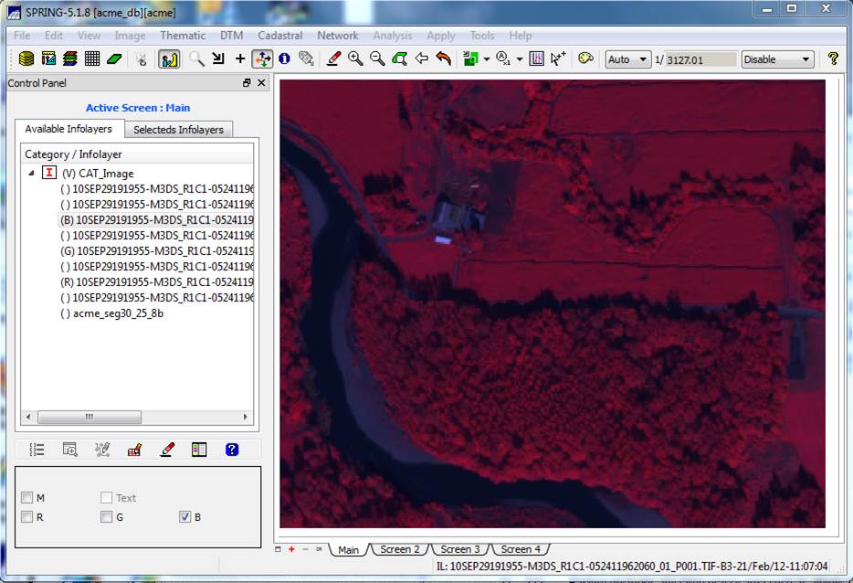
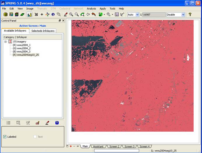
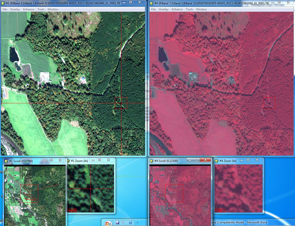
View your image (finally!): In the Available Infolayers window of the Control Panel you will see a list of all eight bands in the image. Highlight band 7 (this is the WV-2 NIR-1 band; see the tech specs at the beginning of this lab), then click the R checkbox in the lower left portion of the Control Panel. This will load band 7 into the red color gun. Then load band 5(recall that this is the red band) in the green color gun (G checkbox) and finally band 3 (recall that this is the green band) in the blue color gun (B checkbox). Your display should now look something like this:

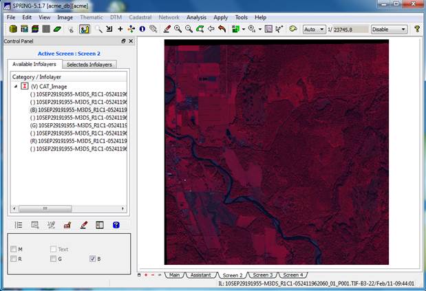
How about that! OK, I know this was seems like a ton of work just to display an image. I don’t know why they make it this hard but they do. I told you that the learning curve on SPRING was steep! Trust me, the segmentation and classification part of SPRING will be easier.

If the image doesn’t fill up the SPRING display window, you might try clicking on the Zoom to Infolayer button . If you’d like, you can spend some time playing around with the other zoom functions but let’s move on.

Back to Outline

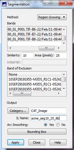
Step 4: Image Segmentation. From the main SPRING toolbar, go to Image-Segmentation

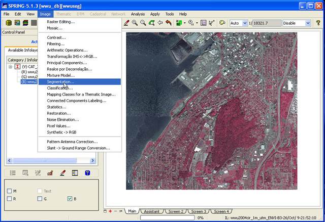
In the Segmentation dialog box, highlight all 8 bands (in the Bands box at the top of the dialog box) by clicking on them one at a time, set the Method box to Region Growing, set the Similarity box to 10 and the Area(pixels): box to 25. This Areas(pixels) sets the smallest region (polygon) that will be delineated in the image. For our Acme, WV-2 image, since we have 2 m by 2 m pixels, a polygon that has 25 pixels will be 10 m by 10 m or 100 m² ; hence our minimum mapping unit is 100 m² . This roughly corresponds to the zone of influence of a single canopy dominant tree. Leave the Band of Exclusion box set at “None.” The idea here is that, if you have one of the layers in your image that represents a portion of the image that you want to exclude from the analysis, you can designate this here. We want to use the entire image so we’ll skip this. In the Output section, leave the Category set to “CAT_Image.” Under IL Name provide a name for this segmentation. This will be a new layer in your image. Something like “acme_seg10_25_8b” might be good. This indicates a segmented image with a similarity of 10 and a minimum region size of 25 pixels, and using all 8 bands. Set the Arc Smoothing checkbox to yes and click on Apply. This takes a while to run.

For the Acme WV-2 image, I want you to do two segmentations. The first using all 8 bands (I’ll call this acmeseg10_25_8b) and the second using just the 4 bands that are similar to TM Bands 1-4 (this would be WV bands 2, 3, 5, 7; see Worldview_bands above) (I’ll call this acmeseg10_25_4b).

Feel free to experiment with different similarity values and minimum area sizes. A higher similarity value means that pixels with less similar brightness values in all band (farther apart in spectral space) will be merged together into the same image segment. This means that you will get somewhat larger image segments with a bit more variability within the image segment. A lower similarity value means that you will get somewhat smaller image segments that are more homogeneous. Since this is a very new technique and a new image from a new sensor, I really do not know what will yeild the best results! No kidding, you are doing original research here!

Depending on your image size and your processor speed, it may take minutes to hours for the segmentation to run. Be patient!

For Acme image (2048 rows and 2048 columns) and all 8 bands, this took about 7 minutes on my machine (dual core 2.9 GHz. Processor and 4 Gbytes of RAM).

For Acme image (2048 rows and 2048 columns) and only 4 bands, this also took about 7 minutes on my machine.

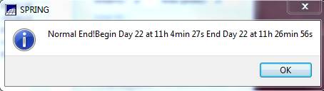
When the segmentation is complete, you will get a message like this:

Back to Outline

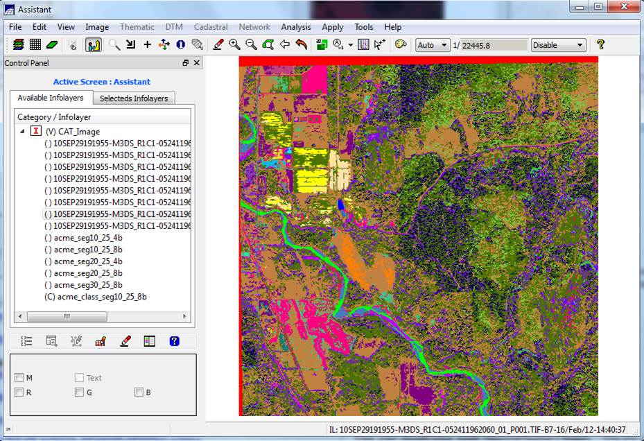
View your Image Segmentation: As soon as you click OK on the message box above, an Assistant window will open. This is essentially a duplicate of the main SPRING window. Go ahead and minimize the Assistant window for now. In the main SPRING window, you will now note that your segmentation layer was added to the Available Infolayers list. Before viewing your segmentation, zoom in by clicking on the zoom button a few times. You should now see something like this:

In the Infolayer section of the Control Panel, click on the acme_seg10_25_8b layer to highlight it, then click on the “Labeled” checkbox in the lower section of the Control Panel. This should result in overlaying the segmentation on the image. It will take a moment to load. If it doesn’t do so automatically, click on the drawing button to display the image with the segmentation overlaid on it.

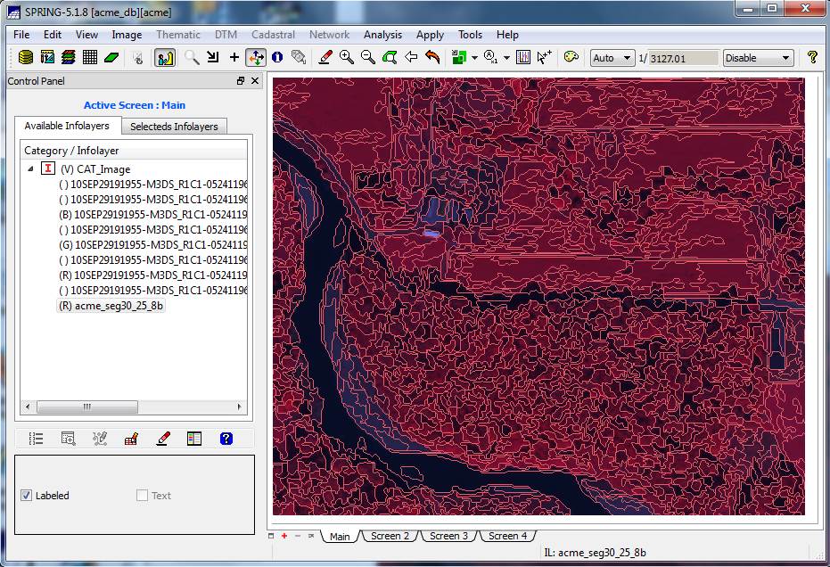
At this point we can see the result of the image segmentation. Note that the individual image segments seem to be fairly homogeneous. This is just what we wanted. Pretty darned cool isn’t it?

Note that if you try to display the entire image by using the Zoom to Infolayer button , it will take a VERY long time to redraw and you will not be able to see much of anything because the individual image segments are indistinguishable at the scale of the entire image. It will look something like this:

Not very interesting.

You can spend some time playing with the various zoom functions. On the main SPRING toolbar, click on the zoom cursor button . Move the cursor into the display window, left click on the upper left corner of the area you want to enlarge, then move to the lower right corner and left click a second time. Now go back up to the main SPRING toolbar and click on the enlarge button . Feel free to play around with some of the other zoom tools, including the roaming cursor button (after clicking on this, move your cursor into the display window, then click, drag and release to move around the image at this same zoom level) and the zoom infolayer button (this zooms you back out to the full extent of the image).

Pretty cool isn’t it? If you would like, you can spend some time playing with the zoom functions but don’t spend too much time here. We have lots more to do!

Back to Outline

Step 5: Classification of Segmented Image: We will now perform an ISODATA unsupervised classification of the image. The individual image segments will be classified on the basis of the mean value of each of the bands for all pixels in the image segment, the covariance matrix and the area of the segment.

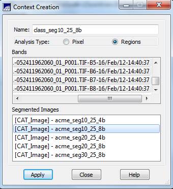
Context Creation: This defines the bands that will be used in the classification and the image segmentation to be used (in the case where you may have run several segmentations based on different similarity and area parameters). From the main SPRING toolbar, go to Image-Classification. In the Classification dialog box, push the Create button. In the Context Creation dialog box, go to the Name: box and enter a name. Something like “class_seg10_25_8b” might be good since we are doing a classification of a segmentation that was created using a similarity value of 10, a minimum area of 25 pixels and using all 8 bands. Of course, you could name it something like “Bob”, but that would not be a particularly informative name now, would it? Under Analysis Type: click on the Regions checkbox (note that “regions” are synonymous with “Image segments”). Under Bands click on each of all 8 bands (or just 4 bands if you are doing a classification using the 4 “TM-like bands; see the table of Worldview_bands above) and under Segmented Images click on our acme_seg10_25_8b segmentation layer. Finally, click on the Apply button.

Back in the Classification dialog box, go to the Contexts box and highlight the context file that we just created (I named mine “class_seg10_25_8b”. You should have only one choice in the Context box.). When you do this, the bands you selected will appear in the Bands box and the name of your segmentation should appear in the Segmented Image box.

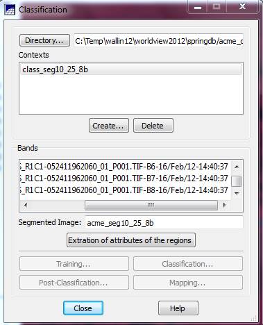
Extraction of attributes of the regions: Now push the Extraction of attributes of the regions button. For each segment (region) in the image, the program will calculate the mean brightness value for each band from every pixel, it will calculate the covariance matrix and it will also calculate the area of each segment. These parameters will be used (below) for the classification. It will take a couple of minutes to complete these calculations (this took about 2 minutes on a computer with a dual-core 3.2 Ghz processors and 4 Gbytes of RAM).

Back to Outline

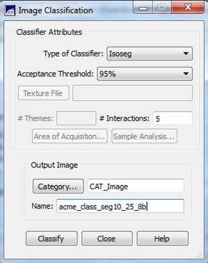
Image Classification: From the Classification dialog box, push the Classification button. In the Image Classification dialog box, go to the Classifier box, select Isoseg (this will perform an ISODATA classification) and change the Acceptance Threshold to 95%. Leave the # Interactions: at 5 (OK, I’m not sure what this parameter does? I suspect that this is a typo and they really mean # Iterations, not # Interactions). Leave the Category as a “CAT Image.” Go to the Name box and enter a name for your classification; something like “acme_class_seg10_25_8b” might be a good choice. Finally, push the Classify button.

The classification process should be complete in a minute or two. Be patient! You may initially get a “Not Responding message appearing at the top of the Image Classification dialog box. When the classification is complete, you should see something like this.

Push OK to close this box and proceed. As soon as you close this box, an Assistant window will appear.

Back to Outline

View your classification result (Spectral/Spatial Classes): You will also note that your result (acme_class_seg10_25_8b in my case) is added to the bottom of the Infolayers list in the Control Panel. It should look something like this.

You can take a look at this, or, minimize the Assistant window, close the Image Classification dialog and go back to the main SPRING display. Go to the Control Panel and scroll down to the bottom of the Infolayers list. You should see your classification result. Click on it to highlight it and click in the Classified checkbox below, then click on the Drawing button . This will show you the same thing that you saw in the Assistant display.

Either way (main SPRING display or the Assistant display), you will now see your spectral/spatial class map. Each region (image segment) will have a solid color and if you look carefully, you will note that some regions have the same color. These represent regions that are in the same spectral/spatial class. The colors in your image may appear a bit different than mine.

Pretty darned cool, isn’t it?

Now do another classifications using (the 4-band image).

When you have finished all of the classifications that you wish to do, we need to get this spectral/spatial class map out of SPRING and back into ENVI so that we can assign these spectral/spatial classes to information classes using the same approach we used for the previous lab.

Back to Outline

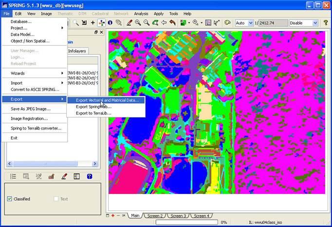
STEP 6: Export your Spectral/spatial Class layer from SPRING. In the Available Infolayers section of the Control Panel, click on the spectral/spatial class map (mine is called acme_class_seg10_25_8b) to activate it. Then, on the main SPRING toolbar, go to File-Export-Export Vectoral and Matricial Data.

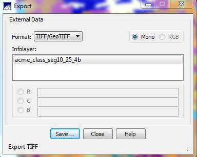
From the Export dialog box, go to the Format: box and select TIFF/GeoTIFF, select Mono, go to the Infolayer box and click on the spectral/spatial class layer and push the Save button.

Back to Outline

STEP 7: Import your Spectral/spatial Class layer into ENVI.

For some reason, ENVI has a problem reading the TIFF file that is created by SPRING. This TIFF file should be a single band file with the values for this band representing the spectral/spatial class values. ENVI can open the file just fine, but it is opened as a 3-band file with the values for the three bands representing the mix of red, green and blue values that create the same appearance that you saw in SPRING. The spectral/spatial class values are lost. There is probably an easy fix to this in ENVI but I haven’t found it yet. Instead, here is a somewhat convoluted work-around.

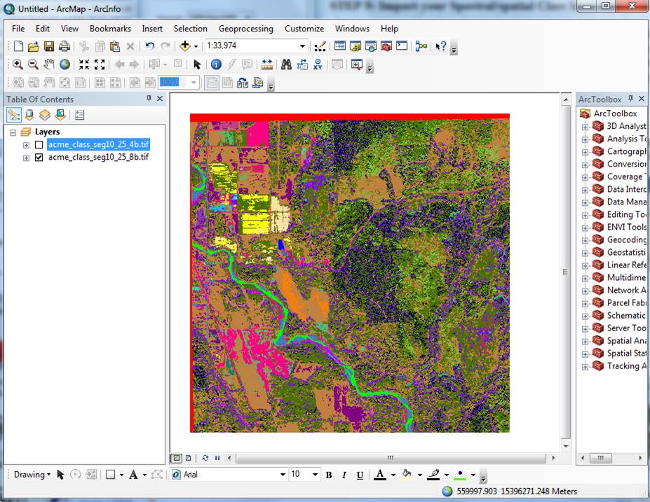
Open ArcMap and create a new project. Then add the TIFF file (both the 8 band and the 4 band) to your project by pushing the “add image button and navigating to the folder containing the TIFF file. After doing so (and assuming the check-box is checked) it should look much the same as it did in SPRING (same colors).

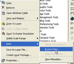
Right-click on the TIFF file and go to Data-Export Data:

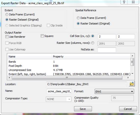
From the Export Raster Data dialog box, specify a Format of ENVI, then select a Location and Name for the output file (I chose to name it acme_clseg10_25_8b.img).

Important Note (2/18/16): Someone just pointed out that in the current version of Arc, the “NoData as:” box in the Export Raster Data dialog box is not blank. The default value appears to be 256. If you take this default, you will get a warning message at some later point (I think in ENVI; not sure) that says something about a problem with your No Data value. I think this is because a value of 256 is out of range for an 8-bit file. Simply dismissing this error message and moving on seems to be OK. However, to avoid this issue, you should set “NoData as:” box to either zero or delete the 256 value and leave it blank.

After doing this, hit Save in the Export Raster Data dialog box.

Now repeat this export process for the 4 band image.

You can minimize ArcMap but leave it open. We will be coming back to it.

Open your file in ENVI. It should contain a single band. In the Available Bands List dialog, right-click on the image and go to Quick Stats to see how many spectral/spatial classes there are in your image. In my case, there are 39 classes (class #0-38) for my 4-band classification and 33 classes (class 0-32) for my 8-band classification. Right-click on the image again and go to Edit Header. You will note that the image has a File type of “ENVI Standard.” Change this to “ENVI Classification” so that we can add a color scheme to the image. When you do this, a dialog box will open asking you to enter the number of classes. After doing so, a Class Color Map Editing dialog box will open. Close this for now; we’ll come back to it. Open this in grey scale in a new display. It should come up with the same colors that you had for this image in SPRING. Now open the original starting file (10SEP29191955-M3DS_R1C1-052411962060_01_P001.TIFF) and load it into a display as an RGB image with the near-IR, red and green bands loaded into the Red, Green and Blue color guns. We want to link these two displays but, before we can, we need to edit the map info in our spectral/spatial class image.

Editing the Map Info: In the Available Bands List click on the + sign next to the Map Info for both images. You will note that the Map Info for these two files is not the same:

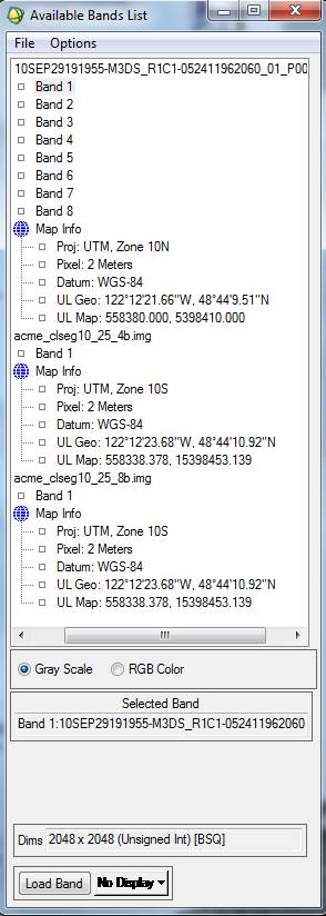
The Map Info for our new classified images is not correct. For some reason, some of this information was lost or corrupted somewhere along the line. Among other things, note that the UL Map northing (the second value) is off. Not sure why but, I’ve noted that SPRING has a habit of adding 10 million meters (10,000,000 m = 10,000 km) to the Northing coordinate. We also need to fix the UTM Zone from 10S to 10N. So, Right-click on Map Info for your spectral/spatial class image and go to Edit Map Information. Click on Change Projection in the resulting dialog box. In the Projection Selection dialog box, change the Zone from 10 S to 10 N. Not sure, but since the software was written in Brazil, maybe it defaults to the southern hemisphere? Leave all the other settings unchanged and click OK

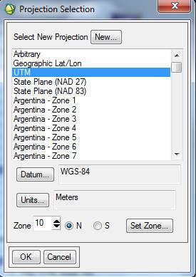
Click OK to close the Projection Selection dialog. Back in the Edit Map Information dialog, the Northing coordinate should have changed (reduced by 10 million meters). You will also note that the coordinates for the UL corner of your classified image are not the same as the UL of your original image. Not sure why, but the classified image produced by SRPING has ~43 or 44 more rows and columns than the original image. You can check this by looking at the header for the original image (2048 samples (=columns) and 2048 lines (=rows)). The classified images seem to have 2091 columns and 2092 rows. The difference in the coordinates for the UL corner are due to these “extra” rows and columns. The images should line up OK now…..I thinks.

Make the same change for your other classification.

Back to Outline

STEP 8: Assign Spectral Classes to Information Classes: You know what to do from here. Open both classified images in ENVI in separate displays. At the same time open the raw TIFF in two different displays; one as a color-IR image (bands 7, 5, 3 into the RGB layers, respectively) and also as a “true color” display (bands 5, 3, 2 in the RGB layers, respectively). Link all three displays to confirm that everything lines up properly. You may need to play around with the enhancements to improve the appearance of these images, especially the color-IR image (I found that a square root enhancement on the scroll window looked pretty good). Move around the images a bit to get familiar with the area.

Recall that the image was acquired in late September. In the true color display, you will note that some of the trees are changing color. These are deciduous trees (mostly red alder, bigleaf maple and cottonwood).

Do your best to assign the spectral classes in each classification to one of the information classes listed below. You should also add a “shadow” class. Unfortunately, we don’t have any ground truth data from this area that we can use to assist with this. I’m anxious to see what we come up with and what the differences are between the 8-band and 4-band classification.

Just to get you started, here is a detail of part of the image:

Young conifer stand; ~15 years old.

~50 year old conifer stand. Some understory deciduous understory vegetation may be visible through canopy gaps.

Do your best to assign the spectral classes to information classes based on visual cues in the images plus your experience with previous labs. We have a very limited set of ground data and I want to save that for an accuracy assessment. We will discuss the image in lab and point out a few more visual cues that can be used. Try to assign your spectral classes to the following information classes

Code	Description
111	Residential
120	Farm Building
141	Road
172	Shrubs
211	Crops
212	Pasture
400	"Recent" Clearcut
410	Deciduous forest
420	Conifer forest
510	Water
620	Nonforested Wetland
740	Rock/Gravel bar/soil

Back to Outline

Step 9: Accuracy Assessment: The folder for this lab (J:\saldata\Esci442\worldview2012) includes an excel file (pcq_lulc_data_acme.xls) with ground truth data. We have ~150 points with LULC Level3 codes that can be used to conduct an accuracy assessment. We also have ~40 PCQ points and we will use these data for a LIDAR lab in a few weeks. Using the data in the Excel file, I have created an ROI file for you to use (test12.roi). This file includes points for each of the 12 information classes listed above.

Return to ESCI 442/542 Lab Page

Return to ESCI 442/542 Syllabus

Return to David Wallin's Home Page