Lab III: Unsupervised Classification with ENVI

Last Updated 1/26/2024

Outline of Document (Click on links to jump to a section below):

Introduction

Procedures:

Step 1: The Imagery

Step 2: Unsupervised Classification

Step 3: Preliminary Assignment of Spectral Classes to Information Classes

Step 4: Use of Ground Truth Data to Aid Assignment of Spectral Classes to Information Classes

Step 5: Classification Accuracy; Generating a Confusion Matrix

Step 6: Area measurements

Step 7: Rule-based Refinement of your Classification in ArcMap

Step 8: Lab Report

Objective: The objective of this lab is to introduce you to the use of unsupervised classification to develop a Land Use Land Cover (LULC) map for our Baker to Bay image. We will also perform an accuracy assessment of our result.

Introduction: In our previous lab, we relied on density slicing to identify different cover types in satellite imagery. As you now realize, this process is rather subjective. This exercise will introduce you to a more objective, statistically based approach to identifying various cover types using a process called Unsupervised classification. Unsupervised classification is a method that examines a large number of unknown pixels and divides them into a number of classes based on natural groupings present in the image values. Unlike supervised classification, unsupervised classification does not require analyst-specified data prior to starting the classification process. The basic premise is that pixels from the same cover type should be close together in the spectral measurement space (i.e. have similar digital numbers), whereas pixels from different cover types should be comparatively well separated in spectral space (i.e. have very different digital numbers). This process can simultaneously utilize data from multiple bands.

The classes that result from unsupervised classification are referred to as spectral classes. Because they are based on natural groupings of the image values, the identity of the spectral classes will not be initially known. You must compare classified data to some form of reference data (such as large-scale imagery, maps, or site visits) to determine the identity or information classes of the spectral classes. Each information class will probably include several spectral classes. Our reference data will come from the site visits done in previous years and new data that you have collected.

It is hard to imagine how the natural groupings of the image values are created in a space that has more than three dimensions. Fortunately, statistical techniques are available that can be used to automatically group an n-dimensional set of observations into their natural spectral classes. Such a procedure is termed cluster analysis by statisticians. In the remote sensing literature, cluster analysis is referred to as Unsupervised Classification. Prior to lab, it will be essential for you to read Chapter 12 in your textbook. Chapters 6 and 7 in the text by David Verbyla will also be useful. As I mentioned in class on several occasions, scanned copies of the chapters from Verbyla (PDFs) are also available on the Canvas site. In addition, you might also take a look at the ENVI online documentation. To get to this, from the ENVI Toolbar go to Help-Contents. Then do a search for ISODATA classification.

Loose Ends: We will be using the ground truth data you collected a week or so ago using the Garmin GPS units. You will need to export these data from Pathfinder Office into a form that we can use for this lab. The procedures for doing this are as follows:

Open Pathfinder Office and go to Utilities-Export. From the Export dialog box, use the browse button to select your “rover” file. This is the file you created in the field. It should have a .ssf suffix. Specify an output folder for your export file. Under “Choose and Export Setup”, select “Sample ArcView Shapefile Setup, then select Properties. Go to the Coordinate system tab and specify UTM, Zone 10 North with a Datum of NAD 1927 (Western United States). Under the Position Filter Tab and the “Include Positions That Are” section, be sure to check the box for “Uncorrected.” We did not differentially correct our data and if the Uncorrected box is not checked, none of your data would be exported. Finally, go to the Attributes Tab. Click on Code Value 1 and be sure that the Position box is checked under Point Features. I’d suggest that you make sure that none of the boxes are checked under General Attributes other than the Position box under Point Features. If any other boxes are checked, this will just export a bunch of information that you don’t really need. Click OK to close the Export Setup Properties dialog box, then click OK again to close the Export dialog box. Now close Pathfinder Office and go to the output folder you specified. You should find three files called LULCII.shp, LULCII.shx and LULCII.dbf. Double-click on the .dbf file and it will open in Excell. If you did things correctly, it will contain only the LULC codes and the UTM coordinates for each point.

Reality Check: Are all of your points realistic? A good way to check this is to overlay your points on an air photo of our study area. Open ArcMap and add an air photo of Bellingham from C:/gisdata/airphoto02. Now add the shapefile you just created. Take a look at each point and see how things line up. When you are satisfied, email me all three of these files to Courtney. We will compiles the data for the class and use these for our accuracy assessment later in the lab.

PROCEDURES

Step 1: The imagery. For this lab we are going to use the Baker-Bay study area that we used earlier this term. All the data for this lab are contained in J:\saldata\esci442\baker_bay_ENVI\imagery.

For our very first lab, I had you use data from July of 2005 for this Baker-Bay scene. For the current lab, I’d like you to use a Landsat 8 image from August 22 of 2017. I looked for a summer 2018 image but all of these had significant amounts of smoke from the wildfires in BC. Using these images would be problematic.

Data from this same area from August of 1988, August of 1992, July of 1995, late September of 2000, July of 2005 and July of 2011 are also available. Note that this Baker-Bay scene is a subset of about 1500 lines by about 2500 columns taken from a full TM scene. A full TM scene is about 9000 rows by about 9000 columns. The 2017 Baker-Bay image is available at: J:\saldata\esci442\baker_bay_ENVI\imagery\bakerbay2017.img. Grab the .hdr file as well (bakerbay2017.hdr). This file contains seven channels (also known as “layers” or “band”).

This 2017 image is from the Operational Land Imager (OLI) that is carried on Landsat 8. All of the other images were acquired using the older Thematic Mapper (TM) or Enhanced Thematic Mapper (ETM) instruments that were carried on the older Landsats. The TM and ETM included six bands with a spatial resolution of 30 m but the newer OLI includes eight bands at 30 m. Here is the comparison:

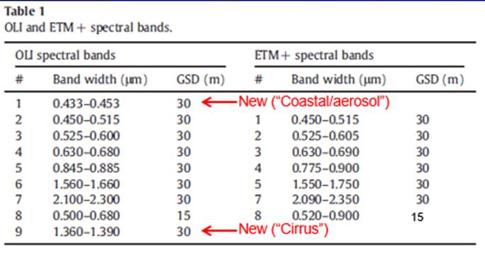
Note that OLI bands 2-7 are similar to TM 1-5, 7. We will be using the 2017 image and OLI bands 1-7 for our classification.

For this lab, we will be using and generating a large number of files. File and folder management will be critical for this lab! For this reason, under C:\temp (where you are working right!? Don’t work directly from your Onedrive or directly from your external storage device!?!), create a Bakerbay folder and a subfolder called Imagery. For me this would look like: C:\temp\wallin\Bakerbay\imagery. Put a copy of the 2017 image (and some of the older images if you’d like) in this folder.

Open the 2017 image in ENVI. Just for fun, you may want to take a look at the older images. Among other things, you will note that the 2000 scene has much less snow than the 1995, 2005 or 2011 scenes. This is mostly due to the fact that the 2000 scene is from late September and the 1995, 2005 and 2011 scenes are from July. The snowpack late in the spring of 1995 was about the same as the late spring snowpack in 2000. Note that the 2011 scene has a bit more snow than the 2005 scene even though both are from July. Another interesting difference between the 2000 scene and the others is the amount of shadow. The sun is much lower in the sky in late September and this creates more shadow. This could complicate a classification effort that involved using the 2000 scene, particularly on north-facing slopes. Finally, you will notice some differences on these four images that reflect land-use changes between 1988 and 2011. Later in the quarter, we will be doing a change detection lab to quantify these changes.

Note regarding ENVI and ArcGIS pro: ENVI has recently entered into a partnership of sorts with ESRI, the folks who provide ArcGIS. Starting with ENVI v4.8 and ArcGIS pro a subset of the ENVI tools are available from within the ArcGIS pro toolbox (assuming that you have paid for both sets of licenses as we have). Those of you who are more familiar with Arc than with ENVI might be tempted to use these tools, instead of working within ENVI.

I’d strongly advise against this.

The ENVI tools available within the ArcToolbox are very limited and the ones that are available provide very few options and limited ability to control the processes. Even worse, it is hard to know what parameters are being used. For example, in the ArcToolbox, if you go to ENVI tools-Image Workflows, you will see an Unsupervised Classification with Cleanup tool. If you open this, you will note that you cannot control the classification process in the way that is available from within ENVI. So, let’s focus on learning to use the more powerful tools that are available from within ENVI.

Step 2: Unsupervised Classification: We will be using the ISODATA unsupervised classification method that I discussed in class. If you haven’t already done so, open the bakerbay2017.img file in ENVI and load an RGB color display as a color-IR image (TM 5, 4, 3 in the red, green, blue color guns, respectively).

-In the Toolbox window, go to Classification Workflow-Unsupervised Classification-Isodata Classification

-In the Classification Input File dialog box, select the bakerbay2017.img file. Click on this file to select it. A bunch of other options will appear. You have the option to work on a Spatial subset (just part of the scene; but we want the Full Scene), use some or all of the bands (we want to use all 7 of the 7 available bands) or to use a Mask to only work on part of the image (but we don’t want to do this.

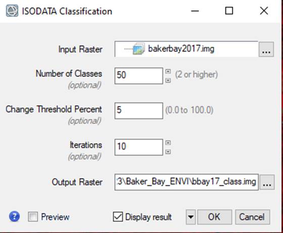
-Click OK and the Classification Input File dialog box will disappear and the ISODATA Parameters dialog box will appear.

-In the Isodata Parameters dialog, set the Number of Classes to 50.

-Set the Change Threshold Percent to 5

-Set the Maximum Iterations at 10.

-Leave all other parameters at the default setting and in the Enter Output Filename box, select a folder and a filename. Something like bbay17_class.img might be good. Click OK.

It will take a bit of time for this to run. Perhaps 5 minutes or so.

Gazillions of calculations are being completed. Be patient. Be amazed. Be glad we have pretty fast computers and recognize that it would have been impossible to do this in a university class just a few short years ago. As it runs, an ISODATA Classifier window will appear that will keep you informed on the progress.

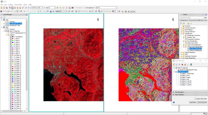
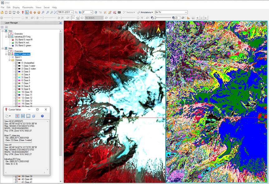
Viewing your classified image: When it finishes, you will see something like this:

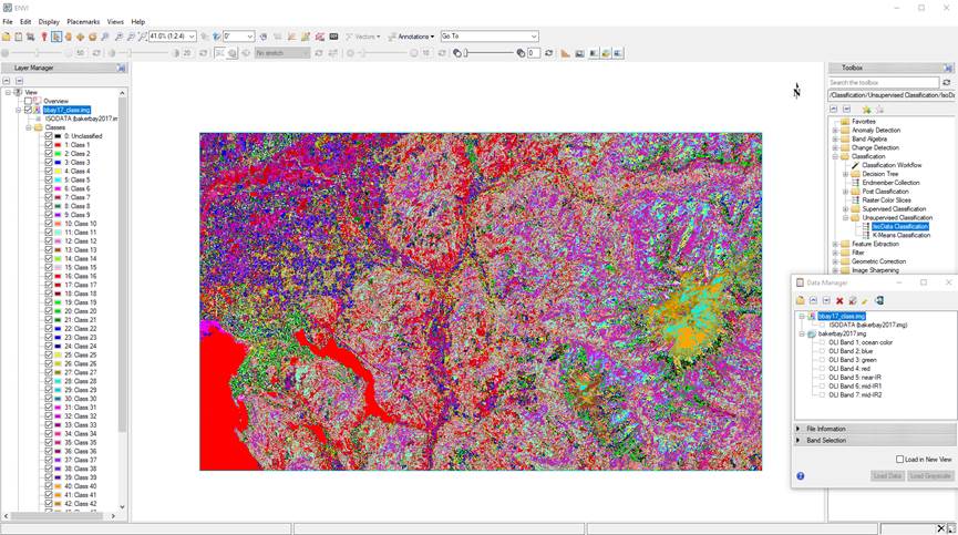
You will note that both your new Isodata output (mine is called bbay17_class.img) and your original bakerbay2017.img file are currently open in the same view. It will be helpful to have these in separate views. To do this:

-If you have not already done so, from the main ENVI Toolbar, go to File-Data Manager (note that, in the above image, the Data Manager dialog box is already open and you will see that both bbay17_class.img and bakerbay2017.img are open.)

-In the Layer Manager window, right-click on bbay17_class.img and go to Remove. Note that this just removes it from this view. It still appears among the open files in the Data Manager window.

-From the main ENVI Toolbar, go to Views-Two Vertical Views.

-Click on your second view (lower one in the Layer Manager window)

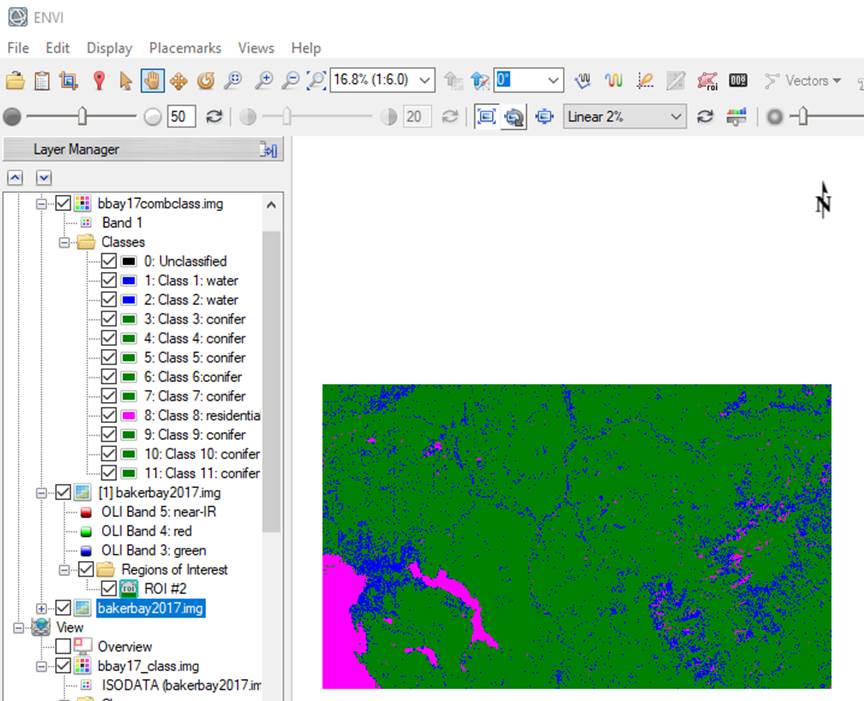
-In the Data Manager window, right-click on bbay17_class.img and Load in Grayscale. Strangely enough, this does NOT result in anything gray. Instead, you will see something like this:

This is just a zoomed in version of what you saw above. By default, ENVI displays Classification results using a Raster Color Slice (you used this in last week’s lab). Each color represents one of the 50 spectral classes that you ask the Isodata classifier to produce. Your task at this point is to interpret your spectral class image (mine is called bbay17_class.img) and assign each of these 50 spectral classes to one of our information classes.

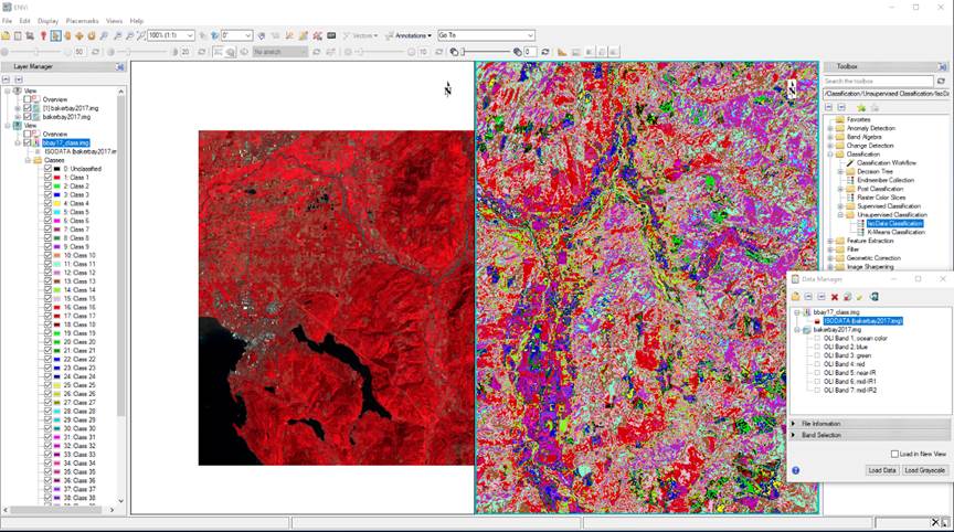
Linking Views: It will be useful to link your two views. To do so:

-From the ENVI Main Toolbar, to Views-Link Views.

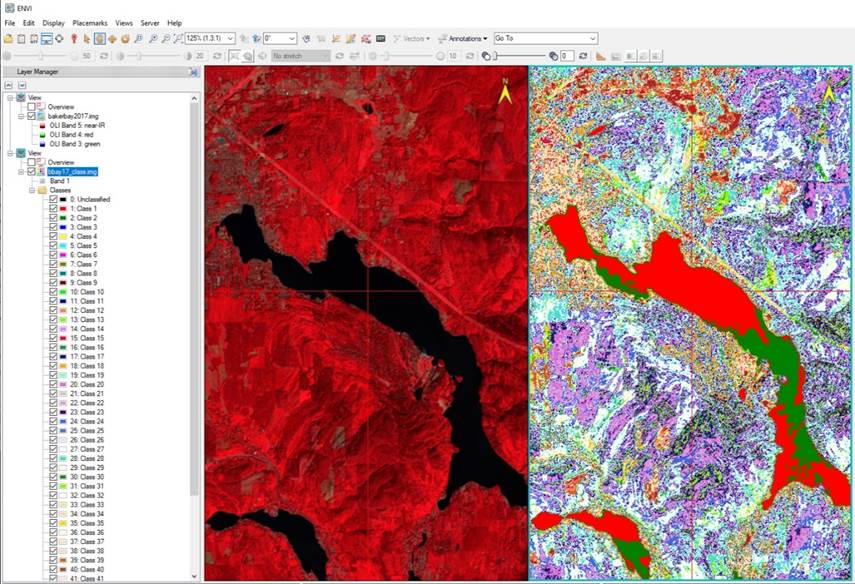
-From the Link Views dialog, select Link All and then click OK. This should result in:

Zooming: Recall that you can zoom in on the image simply using the scroll wheel on your mouse. With the views linked, the zoom both views will be synced.

Moving around the image: Just below, the ENVI Main Toolbar, click on the pan button , then put your cursor in either window, and push and hold the left mouse button to drag the image around (both linked views will drag together).

Step 3: Preliminary Assignment of Spectral Classes to Information Classes: With two sets of views open and linked, you can begin the process of assigning spectral classes to information classes.

-Zoom in on Lake Whatcom (large lake to the east of Bellingham). out to view the full north-south extent of the image at the left (western) side of the image. Look to the north of Bellingham and you will see a small lake. Zoom in on this lake

Just below the ENVI Main Toolbar, select the Cursor Value button and put the crosshairs on this lake.

-In the Cursor Value dialog box, click on the Display Values for All Views button . Click on the northern part of the lake (red in my image).

It should look something like this (but the colors in your map may appear different):

This is Lake Wiser and the grayish line that crosses the lake on the left is the Guide Meridian Road.

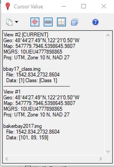
The Cursor Value dialog displays a bunch of information. For each View, the two lines provide the coordinates of the crosshairs (geographic and UTM) and the next two provide information about the map projection. For the bakerbay2017.img file, the last line represents the DNs for the 3 bands that are being displayed. For the bbay17_class.img file, the last line indicates the Spectral Class number; in this case, Class 1 (red color in the right hand view):

-Now zoom out to view the entire north-south extent of the western part of the image.

-Point the cursor to Bellingham Bay. You will note that this is also spectral class #1.

-Point the cursor to Lake Whatcom. You will note that this is also spectral class #1. So this suggests that spectral class #1 probably represents “water.” Also, as you move the cursor around in these water bodies, you will note that the RGB values change somewhat. This indicates that there is some variability within this spectral class but the values are quite similar. Based on our discussion in class and your reading, this is what you would expect.

-Note that the southern part of Lake Whatcom appears green (in my map) and clicking on it with the Inquire Cursor tools shows that it is Class #2, and the Northern part of Bellingham Bay are also Class #2. This also suggests that Class #2 represents another slightly different bit of water.

Let’s explore this “water” class a bit more.

-In the Layer Manager window, right-click on “Class 1” and go to Edit Class Names and Colors

-In the Edit Class Names and Colors dialog go to the Class Names window, click on “Class 1” and edit this to read “Class 1: water”. We want to retain the “Class 1” part of this name for now.

-In the Class Colors window, click on “Class 1” and then click on the little color box adjacent to the “Class 1: water” label below the Class Colors window.

-This will bring up the Select Color dialog box:

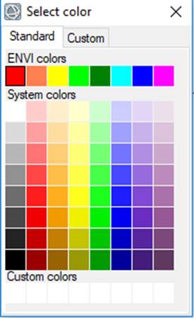
-Select black (humor me for now; I know that this does not seem like a great color choice for water but bear with me), then click OK in the Edit Class Names and Colors dialog

Do the same thing with Class #2. Designate it as Water and change its color to black.

-Not sure why but you may need to relink the two views…..annoying

-You should now see that Lake Wiser, Bellingham Bay, Lake Whatcom and a bunch of other small water bodies show up as black.

Display Group Menu Bar for the spectral class image, go to Overlay-Classification. This brings up the Interactive Class Tool Input File dialog box. Select your spectral class image and click OK to bring up the Interactive Class Tool dialog box. This box shows the default colors assigned to each of the 50 spectral classes. On the Interactive Class Tool menu bar, go to Options-Edit Class Color/Names. In the Class Color Map Editing dialog box, click on Class #1. On the Color drop-down, go to Colors1-20 and select black, then click OK in the Class Color Map Editing dialog box. Back in the Interactive Class Tool dialog box, you will note that the color assigned to Class #1 had now changed to black but there has been no change in the appearance of the display. Click in the “On” box next to Class 1 and, back in the display window, you will see that Wiser Lake, Bellingham Bay, Lake Whatcom and all of the other water bodies have turned black. In the Scroll Window, grab the scroll box

-Now zoom out and move to the right side of the image (the area on the west flanks of Mt. Baker). You will now note several large patches of “water” in this area. Click on a few of these to confirm that they are in “Class 1: water” or “Class 2: water” in bbay17_class.img. By looking in the color-IR display, you will see that these patches of “water” are actually the shadows on steep NW facing slopes of several large clouds. These shadows are also spectral class #1 or #2 and are now mapped as “water.” In other areas, you may see that shadows on the north facing sides of several mountains also are now classified as “water.” This is a problem. This is an example of a case where a single spectral class includes more than one information class.

Let’s move on to another cover type. However, before we do, let’s go back to the Layer Manager window, right-click on “Class 1” and go to Edit Class Names and Colors and let’s give this class a more appropriate color.

-In the Edit Class Names and Colors dialog and the Class Colors window, click on “Class 1: water” and then click on the little color box adjacent to the “Class 1: water” label below the Class Colors window.

-This will bring up the Select Color dialog box. Select the color blue (good color for water), then OK.

Yes, we’ve established that spectral Class 1 is really a “Water/Shadow” class but let’s go with “Water” for now.

- Do the same thing for Class 2 which is also water.

Urban/Rock: OK, now put your cursor on this location on the north side of Mt. Baker:

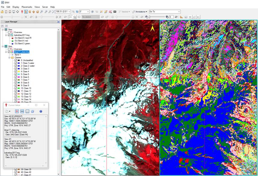
In the color-IR display, this appears to be an area of bare, exposed rock above treeline and below the snow fields. The Cursor Value dialog box indicates that this is mostly spectral class #44. Go to back to your Interactive Class Tool dialog box.

-In the Layer Manager window, right-click on “Class 44” and use the procedure we used for Class 1 to give Class 44 a color of black.

-No idea why but it appears that you need to re-link the displays after doing this @#$#@!!!

-In the Layer Manager window, you can check and uncheck class 44 to turn the black on and off to confirm the extent of this spectral class. You will note that many, but not all, of the rocky areas on Mt. Baker are also in Class 44 and are apparent as you check and uncheck Class 44. This seems reasonable.

-OK, now zoom out and move the image so downtown Bellingham is in view. Zoom in on downtown Bellingham. You will now see that there are now scattered bits of black through much of the downtown area. Check and uncheck Class 44 to help you visualize this:

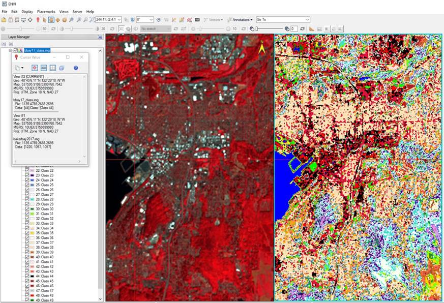
As you can see, in the Bellingham area, spectral class #44 seems to include roads and other features in the urban and suburban area. You might argue that this is another case where a single spectral class includes more than one information class. On the other hand, you might argue that rocks are rocks (apologies to the geologists…..) but some happen to be on Mt. Baker and some are in downtown Bellingham. This gets at the issue of land USE vs. land COVER. The land COVER in both Bellingham and on Mt. Baker is “soil/rocks” (with cement being a sort of rock-like substance) but the land USE is different. In this case, the rocky stuff in downtown Bellingham might go into an “Urban” class but the areas in spectral class #44 that are not in Bellingham might go into a “bare soil/rock” class. This later class might be found in lots of rural and wilderness areas. It might be nice to be able to separate these urban and suburban rocks and soil from alpine rocks and soil. How could we do this? Any ideas?

One way might be to use some information from other GIS data layers. In the case of our urban/alpine problem, one topographic feature that would help to separate these two classes is elevation. Another approach might be to use a roads layer. Any rocky areas near a road may represent the “urban” class but rocky areas that are not near a road might to into the “bare soil/rock class.” In the case of our water/shadow problem a topographic attribute that would separate these two classes is %slope. Water surfaces will have a slope of zero but shadows on steep north-facing slopes will have high % slope values. We will get back to this issue later. No classification will ever be perfect. Later in this lab, we will consider ways in which slope and elevation might be incorporated into your classification. Let’s proceed with the process of assigning all spectral classes to an information class. NOTE THAT MOST INFORMATION CLASSES WILL INCLUDE SEVERAL SPECTRAL CLASSES! Some spectral classes will contain more than one information class (such as water/shadow).

Before we move on to other spectral classes, go back to the Layer Manager window and, using the same procedure we used above, go to Class #44 and edit the class name to something like “Class 44: urban/soil/ rock” and give it a color that you like. For now, leave the “Class 44” as part of the name.

Step 4: Use of Ground truth Data to Aid Assignment of Spectral Classes to Information Classes: At this point, you could use your knowledge of the study area to assign each spectral class to an information class. This approach is common, however, since we have a large set of ground truth data, we can use it to help us with this task. The ground truth data are contained in J:\saldata\esci442\Baker_Bay_ENVI\ground_truth\lulc_refdata2019.xls. Get a copy of the entire \ground_truth folder and place it in your workspace in C:\Temp. Open the lulc_refdata2019.xls file. The file contains over 2000 points collected by students from previous years and each have been assigned to a Landuse-Landcover code (see Table 21.1, page 587 (if using 6^th edition) of your textbook). Note that, in this table, I have come up with a set of hybrid codes that are a mix of Level II and Level III LULC codes. The Anderson Level II codes in this table range from 11 to 91. The Level II/III codes range from 110 to 910. I have collapsed some of these together to come up with 11 classes. These are the potential information classes that we will try to identify in our classified image. Note that this is an overly optimistic goal and we may end up merging some of these information classes.

For the 2017 data, I’ve done something a bit different and this dramatically increases our sample size. For each of the points you provided, I calculated the coordinates of the eight cells surrounding this point by adding or subtracting 50 m from the X and or Y coordinate that you provided. For example, for the cell to the lower left of the cell you gave me, I calculated:

New Y = Your Y – 50

New X = Your X – 50

So, although you provided me with 190 GCP coordinates, I was able to generate an additional 1520 GCP points. This nearly doubles the sample size that we had to work with last year.

Table 1:

Anderson Level II LULC Codes	Simplified LULC Codes for ERDAS	Modified Level II/III LULC code for ENVI	Class description
0	0	0	Background
11	1	110	Residential
12 - 17	2	120	Urban or Built up lands
211	3	211	Ag. Pasture/Grass
212-24	4	212	Crops
31-33			Does not occur here
40	5		"Recent" clearcuts; anything cut since 1972
		401	1973-79 clearcut from Boyce
		402	1979-85 clearcut from Boyce
		403	1985-88 clearcut from Boyce
		404	1988-92 clearcut from Boyce
		405	1992-95 clearcut from Boyce
		406	1995-2000 clearcut from Grace
		407	2000-2002 clearcut from Cohen
		408	2002-2005 clearcut from Wallin
		409	2005-2011 clearcut from Wallin
41, 43, 61	6	410	Deciduous forest
		411	2011-2017 clearcut from Wallin
42	7	420	Conifer forest
51-54	8	510	Water
71-77	9	710	Soil/rock
81-85	10	810	Alpine veg., non-forest
91, 92	11	910	Snow/ice

Table 2: Merged LULC classes for use in this analysis

Output Class	Class Description w./LULC codes
1	Residential; 110
2	Urban; 120
3	Pasture; 211
4	Crop; 212
5	Clearcut_05_17; 409 and 411
6	Mixed; 406, 407, 408, 410
7	Conifer; 401, 402, 403, 404, 405, 420
8	Water; 510
9	Rock; 710
10	Alpine; 810
11	Snow; 910

I did quite a bit of work to screen these data for errors (“Quality Control”). The data from previous years is on the “lulc2018QC” worksheet. We want to use about half of the data to aid in assigning spectral classes to information classes (a “training” data set) and use the other half of the data to perform an accuracy assessment (a “test” data set). ENVI doesn’t make it particularly easy to work with a dataset like this. I’ve done quite a bit of preliminary work for you. Here is what I’ve done. In the Excel file, you will note that there are a large number of worksheets. Starting with the “lulc2018QC” worksheet, I have:

1. Added an additional column using the RAND() function in Excel. This function generates random numbers ranging from 0.0 to 1.0.

2. I then sorted the points by these random numbers.

3. I then took all points with random numbers from 0.0 to 0.50 (representing about 50% of the data) and copied this to a new worksheet that I called “training.” I took the remaining data, with random numbers ranging from 0.50 to 1.0, and copied this to a new worksheet called “test”.

4. On both the “training” and “test” worksheets, I then sorted by the level II/III LULC codes, then copied the data for each code to a separate worksheet. This created a large number of worksheets, half for the training data and half for the test data. These worksheets have names like “train110, train120,…train910” and “test110, test120,….test910.”

5. Each of these worksheets were then saved to separate tab-delimited .txt files: train110.txt, train120.txt,….train910.txt and test110.txt, test120.txt,…test910.txt.

6. Finally, I brought all of the “trainxxx.txt” files, one at a time, into ENVI to create a “Region of Interest” file that contains the 11 classes listed in Table 2 above. I did the same thing with the “testxxx.txt files.

Cross Tabulation; An Objective Approach for Relating Information Classes and Spectral Classes: We now want to cross tabulate our spectral classes and our information classes. For each spectral class, we’d like to know with which information classes it is most commonly associated. Some spectral classes will be unambiguously associated with a single information class. In other cases, a spectral class may be associated with multiple information classes. Here is how we obtain this information. Back in ENVI:

-Go to the Layer Manager window and right-click on your bbbay17class.img file and select New Region of Interest

-In the Region of Interest (ROI) Tool dialog, go to File-Open and navigate to your ground_truth folder and select “train2019QC_11class.roi”.

-In the Data Selection dialog, select your bbay17_class.img file, then click OK.

-Back in the Region of Interest (ROI) Tool dialog, go to Options-Compute Statistics from ROIs.

-In the Choose ROIs dialog, click on Select All Items, then OK

-After watching a bunch of ROI Statistics process status windows scroll by,…

….you will see the ROI Statistics View: bbay17_class.img dialog box,

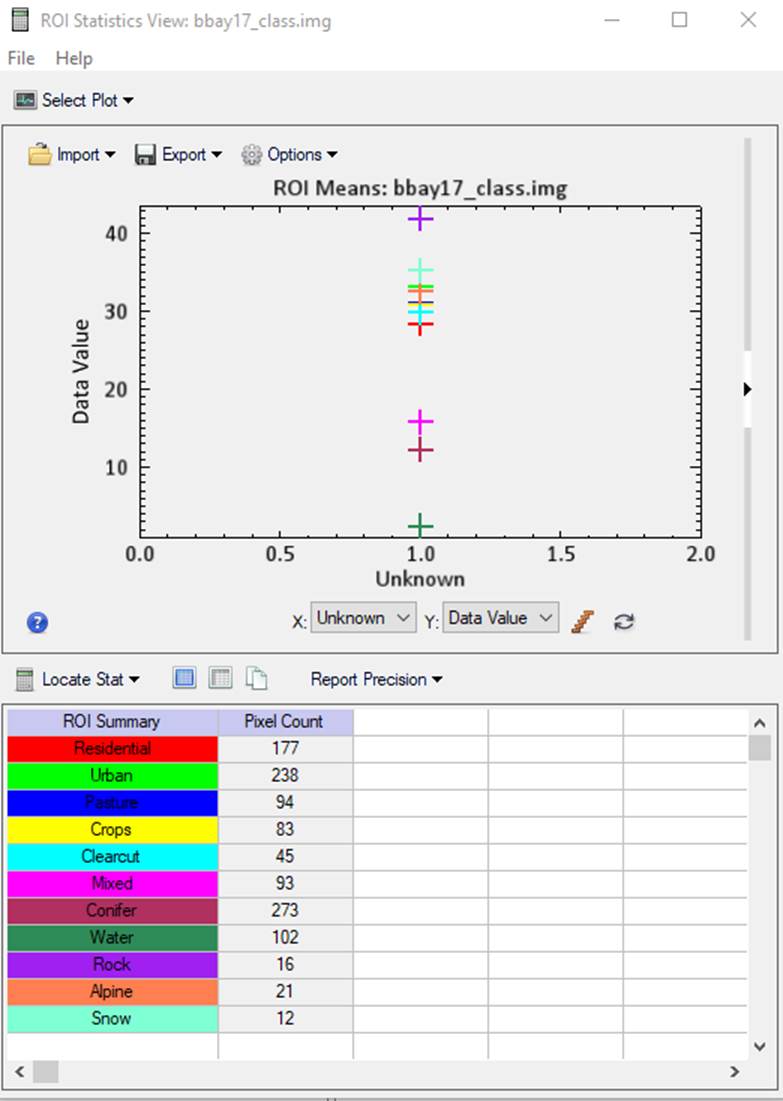
I don’t find the Plot in the top of this dialog box to be particularly useful. What is useful are the statistics in the lower panel (Scroll down to see). In it, you will see a breakdown of the number of pixels of training data you have for each LULC class from Table 2 above. If you use the slider in this window to move down a bit, you will first see a breakdown of results for the “Residential” class. There are columns for “DN” and “Count.” The DNs represent the spectral classes in your image. The “Count” represents the number of Residential training pixels you have for each spectral class.

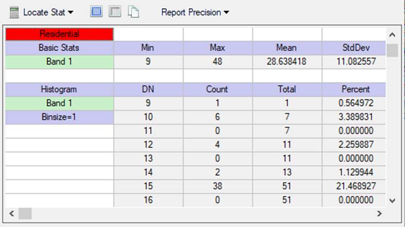
In this case, there are no “residential” training sites in spectral classes 1 through 8. Spectral class#9 is the first to contain any “residential” training sites (and there is only 1 of them). As you scroll down in this panel, you will see that there are 42 residential training sites in spectral class #34. There are residential training sites in other spectral classes as well (including quite a few in classes 15, 18 and 37). The columns to the right of the “Count” column (“Total,” “Percent,” and “Acc Pct”) are not relevant at this point. If you continue scrolling down, you will see this info for the other 10 LULC classes.

We would like to get all of this information, including the info for the other 11 LULC classes, into an Excel file to work with it a bit. To do so:

-In the ROI Statistics View: bbay17_class.img dialog, go to File-Export to Text File.

-In the Export to Text File dialog, select a folder and filename. A good name might be something like “bbay17_crosstab.txt”

- Alternatively, you can copy the statistics with the blue box next to the “Locate Stat” button and press the copy button (button with two sheets of paper) and paste the information into Excel.

-Now you can bring this into Excel for some manipulation. The formatting on this dataset is not ideal. You will need to manually edit this file quite a bit to get it into a useful format. Start by creating a table on a new worksheet that looks like this:

Table values are # of training sites in each spectral class
	Information Class
Spectral
Class	residential	urban	pasture	crops	clearcut	Mixed.	.	.	.	.	.	.	alpine	snow/ice	Total#Pts
1
2
3
4
5
.
.
.
.
.
.
.
50
Total#Pts

Then, start bringing in the data for each information class, one at a time, into this table that you have created.

Yes! I know this is a somewhat annoying editing task! But it will be very helpful. When you have completed this task, compare your table with a couple of your neighbors just to be sure that you have not made any errors. We should all have the same results. When you are confident that you have this compiled correctly, use this information to help you decide which spectral classes to assign to each information class.

Problem Information Classes: You will undoubtedly run into conflicts. Here are the major ones you will encounter:

1. Urban vs. soil/rock: We’ve already discussed this one. Do the best that you can but recognize that, later in our analysis, we will explore the use of other GIS layers to help us separate these two classes.

2. Note that, in the lulc_refdata2019.xls file, I’ve included data for a large number of forest categories. This is a reflection of my interest in forest management and also a recognition that forestry is a major land use category in our region. I have data for stands that were harvested during ten different time periods. I also have data for some stands dominated by deciduous trees and stands dominated by conifers. Recognize that, following a timber harvest, the site will mostly be covered by bare soil, exposed rock and logging slash for a short period of time (a few months to perhaps 1-2 years). The site will then be dominated by shrubs and deciduous trees for a time (perhaps 3-15 years depending on site conditions and management). After that, the site will probably be dominated by conifers until it is harvested or it burns in a wildfire. In riparian zones, deciduous trees can dominate a site for perhaps 50-80 years before conifers replace them. In upland sites, deciduous trees and shrubs will be overtopped by conifers much more quickly. So this suggests that:

a. More recent clearcuts may be confused with bare soil/rock, the agricultural classes (crops and pasture) and the alpine class. Later in our analysis, we may be able to use elevation to separate these classes. Agriculture typically only occurs at lower elevations in our study area (<200m), forestry occurs at middle elevations and alpine areas only occur above treeline (>1500 or 1700m).

b. Older clearcuts may be confused with conifer and deciduous. In the ROI, I have collapsed the various forest categories into just three: Clearcut (harvested between 2005 and 2017), Mixed (including clearcuts harvested between 1995 and 2005 as well as stands dominated by Deciduous trees) and Conifer (including pre-1995 harvests as well as other conifer-dominated stants).

3. Based on the class merger described in 2b. you have 11 class: residential, urban, pasture, crops, clearcut, mixed, conifer, water, rock, alpine, snow.ice and a 14^th class that I had to add for this image, “clouds”

Use your cross tabulation to assign as many spectral classes as possible to an information class. There will be a few spectral classes for which there are no training sites. That’s OK, we’ll come back to these. Now go back to ENVI.

-In the Layer Manager window and the View containing your “bbay17class.img” file,

-Right-click on one of the class names and go to Edit Class Names and Colors. Come up with a color scheme (unique color for each LULC class) and, using the results from your cross tabulation, assign class names to each spectral class. (Note: at this point, I’d suggest that you retain the class numbers; just add a descriptive name to each class number. e.g., “Class 1; water.”)

-Assign the color black to all spectral classes that you are not sure about.

-When you are done, click OK to close the Edit Class Names and Colors dialog box.

Take a look at your image. How does it look? You can click on individual check-boxes to toggle between the colors you assigned and the default color scheme for an individual spectral class. Move around the image to get a feel for the result. As you do this, it is helpful to have your classified image and a color-IR image open at the same time and have the two views linked.

Using Spatial Context to Modify Classification: You undoubtedly had a few spectral classes for which you had little or no training data. In other cases, you may have had a “tie vote” between classes. Uncheck the boxes for all of these “unknown” classes except one. For this one remaining unknown, alternately check and uncheck the box to figure out where it is in the image. Try to figure out what the spectral class represents on the basis of context; to what information class have the surrounding areas been assigned?

NOTE: It is very important that you assign at least one spectral class to each of the information classes!

In addition to referring to the color-IR or true color version of the Landsat image, you can also refer to recent air photos of the area that are available through Google Earth. An easy way to view this is to center your cursor (in ENVI) on an area of interest. Then, from the Display Group Menu Bar, go to Tools-SPEAR-Google Earth-Jump to Location. This will bring up a recent air photo of the area. If you do this, note the date of the imagery that shows up in Google Earth. It may or may not be close to the date of our August 2017 Landsat image.

Save Your Work: After you are confident of your class assignment, save your color assignments and class names. Do so in the Interactive Class Tool Menu Bar by going to File-Save Changes to File. You will be asked to confirm this action because this information is stored as part of the header and this color scheme will always be associated with your spectral class image whenever you reopen it.

Combining Classes: After you are confident of your class assignments we will now create a simplified image which combines all spectral classes that are in the same information class. Instead of having 50 classes (many of which represent the same thing), the resulting image would have only 11. To create this simplified image:

-In the Toolbox search box, enter Combine Classes and click on this tool

-From the Combine Classes Input File dialog box, select your “bbay17_class.img” (or whatever name you used for this file). Then click OK.

-The Combine Classes Parameters dialog box is somewhat confusing. It will look something like this:

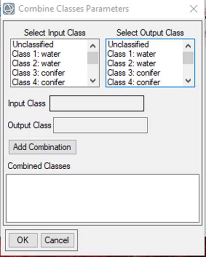
Note that, by default, the Output Class names are identical to the Input Class names. This is confusing and unfortunate because, to make one of the later steps easier, it will be VERY helpful to assign output classes IN A PARTICULAR ORDER. That is, your output class #1 should be Residential, class #2 should be Urban, etc. Like this:

Table 2:

Output Class	Class Description w./LULC codes
1	Residential; 110
2	Urban; 120
3	Pasture; 211
4	Crop; 212
5	Clearcut_05_17; 409 and 411
6	Mixed; 406, 407, 408, 410
7	Conifer; 401, 402, 403, 404, 405, 420
8	Water; 510
9	Rock; 710
10	Alpine; 810
11	Snow; 910

As shown above, the default output class name for Class 1 in my case is “Class 1: water.” I want to assign all my spectral classes for residential lands to output Class 1 (which has the default name of “Class 1: water.”). At this point, I’ll just have to ignore the “water” part of this output class name (we’ll come back later and change this name). So I’ll do this:

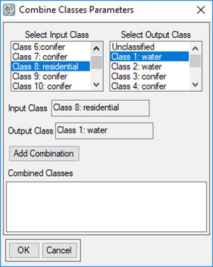
In my case, spectral class #8 was the first that I chose to put into the Residential output class, which unfortunately at this point has the name “Class 1: water.” Again, at this point you just have to ignore the “water” part of the output class name. Just keep telling yourself that Output Class 1 is “Residential” not “Water.” Yes, I know that this is confusing. After entering the Input and Output classes, click on Add Combination to get this:

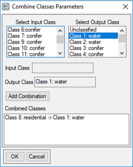
Continue by assigning all spectral classes to an output class using the output class assignments given in Table 2. After you have assigned all of the input classes to an output class, click OK in the Combine Classes Parameters dialog box.

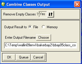
This brings up the Combine Classes Output dialog box.

IMPOTANT: Set the Remove Empty Classes box to Yes, This insures that your new file will have 11 classes rather than 50 classes, most of which would be empty.

Set the Output Result to- File and specify a folder and filename. Note: I have just discovered that, for reasons discussed below, you should be sure to give your file a .img extension. If you fail to do this, Arc will not recognize the file as a raster image file. Then click OK.

The resulting image should open in your active View. When it does, all the class names and colors will be goofy. Like this:

You will now need to go in and edit all the class names (from Table 2 above) and colors to generate something that looks like your bbay17_class.img file.

This is where you can fix the class names (I edited my “Class 1: water” name to “Residential” following the class numbers/names in Table 2) and assign the same colors that you used for your spectral class image. After you have done this, your combined classes image should appear exactly the same as your spectral class image, however, if you right-click in the image window and select Quick Stats.., you will note that the image only has 11 classes, not the 50 classes that your spectral class image has.

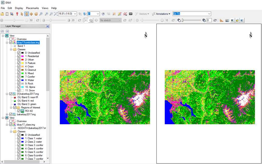
After doing so, both your 50 class image and your 11 class image should looks the same:

Note: A number of people seem to have somehow corrupted their combined classes image at this point. I’m not certain how but here is one possibility. At this point, you probably have your combined classes image displayed and it is tempting to think that you may have to save your image. THIS IS NOT NECESSARY. Here is one way that you could accidentally corrupt your image. If you go to the Display Group Menu Bar and then go to File-Save Image as-Image File, THIS WILL CORRUPT YOUR IMAGE IF YOU SELECT AN OUTPUT FILENAME THAT IS THE SAME AS YOUR INPUT FILENAME. What you would be doing is saving your single band, 11-class image as a 3-band RGB file. In doing so, you would lose all of the information in your combined classes image and your filesize would go from about 3.7 Mbytes to about 11.1 Mbytes. SO DON’T DO THIS.

Step 5: Classification Accuracy; Generating a Confusion Matrix: We are now ready to check the accuracy of our classified image. To do this, we will use the “test” data that we set aside from our ground truth dataset. Go back and take another look at your “lulc_refdata2019.xls file. Recall that this file contains a series of worksheets labeled “test110, test120,….test910.” Note that I merged many of the forest classes to create an ROI file with just 11 classes (test2019QC_11class.roi). So:

-In your view that holds the combined classes file, right-click on your combined classes image and go to New Region of Interest.

-From the Region Of Interest (ROI) Tool dialog box go to File-Open and select the “test2019QC_11class.roi” file in the ground_truth folder and click on Open

-In the Data Selection dialog box, select your combined classes image and click OK

-Select Base ROI Visualization Layer) again select your combined classes image and click OK

-In the Toolbox search window, enter Confusion Matrix and select the Confusion Matrix Using Ground Truth ROIs

-In the Classification Input File ((Confusion Input File)) dialog, select the combined classes image and click OK

((-In the Data Selection dialog box select your combined classes image and click on OK))

-In the Match Classes Parameters dialog box, you will see a Select Ground Truth ROI box and a Select Classification Image box. The software will try to match these classes up and, if you used similar names in each, it will probably be able to do so. If the names you used are different, you may need to manually match these up. In my case, the software was able to match up every class.

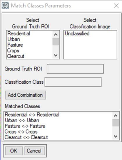
So, I just need to click on OK.

-In the Confusion Matrix Parameters dialog box, uncheck the Percent box, leave the Pixels box checked and Report Accuracy Assesment at Yes. Then click on OK.

-In the Class Confusion Matrix dialog, go to File-Save Text to ASCII

-In the Output Report Filename dialog, choose a folder and filename, then click OK.

Open your Confusion Matrix in Excel: We now want to open this file in Excel and manipulate it a bit. When you open it in Excel, you are asked for guidance; Excel needs to know how to put things into cells. Opening it as a “Fixed-width” Format should bring it in OK but, if not, try the “Delimited” option. After you bring it in, you will need to manipulate it a bit to create an Error Matrix (ENVI refers to this as a “Confusion Matrix”). Refer to your text, Chapter 13, sections 13.4 and 13.5 (beginning on page 354) for guidance. In your case, the columns in your table represent the Reference Data and the rows represent the Image Data (the example in the text shows the reference data in the rows and the image data in columns). Calculate the Producer’s and User’s Accuracy and the Overall Accuracy (Percentage of all reference pixels correctly classified). Note that you should get a copy of my excel file “sample_error_matrix_2017” that is located in the ground_truth folder. Dropping your data into this excel file will do much of this work for you. In addition to calculating User’s, Producer’s and Overall accuracy, it will also enable you to examine how collapsing some of the classes (settling for fewer than 11 classes) might impact your classification accuracy. You should also read about Cohen’s Kappa statistic. This Error Matrix should go into your lab report. Your table should look something like this:

Table 3:

Predicted	Ground Truth (Reference Data)							Row		User's
Class	Residential	Urban	Pasture	Crops	………..	Alpine	Snow	Total		Acc (%)
Unclassified
Residential
Urban
Pasture
Crops
Clearcut
Mixed
Conifer
Water
Rock
Alpine
Snow
Column Total									Total Samples
									Total # Correct
Prod Acc (%)									Overall Accuracy

After looking at your results, you may choose to go back and tweak your classification a bit to reassign some of your spectral classes to different information classes. Don’t go overboard with this! A classification accuracy over 70% is considered quite good. With 11 classes (the 13 from my test2018QC_13class.roi, plus shadow….for which we have no test data) your accuracy will probably be lower than this. You may decide to combine some of your information classes to achieve a higher accuracy. In particular, you may choose to combine urban and rocks and/or combine deciduous and conifer forest. You should look at my Excel file “sample_error_matrix_2017.xls” (this file is located in the folder for this lab: J:\saldata\esci442\baker_bay_ENVI\ground_truth) for one example of how you might do this. If you have the same information classes in the same rows and columns as I do, you can drop your data into this table to see the effect of collapsing the same classes that I did. Your results will be somewhat different than mine depending on how you assigned spectral classes to information classes.

Step 6: Area measurements. With your combined classes image opened in a display window, you can right-click in the Layer Manager window and go to Quick Stats. This will bring up the Statistics Views display window. In the lower portion of this window under “Histogram”, the “DN” values are the individual information classes (Class 1 is “Residential” if you followed the instructions in Table 2 above) and the “Count” indicates the number of pixels in each class. You can go to File-Export to Text File, bring this file into Excel and calculate the area in each information class. VERY IMPORTANT NOTE: The pixel size in this image is 25 meters by 25 meters. As you know, Landsat TM data normally has a pixel size of 30m by 30m but the raw TM data was resampled to create this Baker-Bay image.

Step 7: Rule-based Refinement of your Classification in ArcGIS pro: We will now use several other GIS layers to do some rule-based modeling to further refine our classification. Some of you may be very familiar with ArcGIS pro and other may have no experience with it. No problem; I’ll walk you through it. Begin by opening ArcGIS Pro. **If it asks for a sign in, click sign in with organization and type in wwu before you sign in. This will bring up an interface that looks like this:

Select “Map”. You will then be asked to create a New Project. Select a Location and a Name. It will chug for a moment and then bring up something like this:

Adding Data layers: Click on Map, then go to Add Data. You can bring your ENVI file directly into ArcGIS pro. Warning: I just discovered that Arc seems to refuse to acknowledge/recognize your ENVI combined class image UNLESS you gave your filename a .img extension. If you didn’t do this originally, simply go into Explorer and rename the file to give it a .img extension. After doing this…. You will be asked if you want to build Pyramids and calculate statistics. Pyramid files are something that enables Arc to zoom in and out much more quickly. Since this is useful, say “Yes” when asked. It will only take a few seconds to create each Pyramid file. Say OK. It should come in with the colors and class names that you specified within ENVI.

You should also add the % slope (bbay_slope.img), elevation in meters (bbay_elevm1) and roads layer (roadbuf100). Each of these are in the Baker_Bay_ENVI folder that you copied from the J:/ drive. Say yes to calculating statistics for each of these.

Note: the elevation and roads layers are Arc grid files. For those of you who are not Arc-savy, you will note that “bbay_elev_m1” and “roadbuf100”will look like folders in Windows Explorer. Go ahead and grab this both folders along with the “info” folder and place BOTH of these in your working directory. The “info” folder include files that relate to the roads and elevation layers. If you fail to copy the Info file, you will run into problems.

You can check and uncheck each of these layers to view them.

On the roads layer, all pixels within 100m of a road have a value of 1 and all other pixels have a value of 0. You can toggle each layer on and off by clicking on the check-box in the list of layers (left-hand window in the ArcGIS pro display).

Adding A Custom Toolbox: With help from Stefan Freelan, I have created several models (or “toolboxes”) for you to use. To load these models, on the main ArcMap toolbar, go to Tools-Options. Then go to the Geoprocessing tab. In the My Toolboxes section, enter the folder that has served as your workspace for this lab. Then click on Apply and OK to close this window.To insert the toolbox click the “Insert” tab on the ribbon on the top of ArcGIS pro. Then, click the red toolbox button and Add Toolbox to add you NestedConModels.tbx file.

Generate Statistics: Before you can run these models, you need to “generate statistics” for your ENVI file within Arc. I’m not sure exactly what Arc is doing but it seems to be critical to enable the models to run. So, here is what you do. In the ArcToolbox, search for Calculate Statistics. This will bring up the Calculate Statistics dialog box.

Click on the folder icon and specify your combined classes image as the Input Dataset. Then click Run. Now you should be able to run the models using the following instructions. Note that, after running the Calculate Statistics tool. If a second copy of your combined classes layer shows up in the table of contents (it may not have the .img suffix on the filename but it should otherwise appear identical to your original combined classes .img file), you can go ahead and delete it by right-clicking on the name and going to Remove.

Go to the Catalog tab on the lower right and expand the Toolboxes icon. This will reveal the NestedConModels tools that you added above.

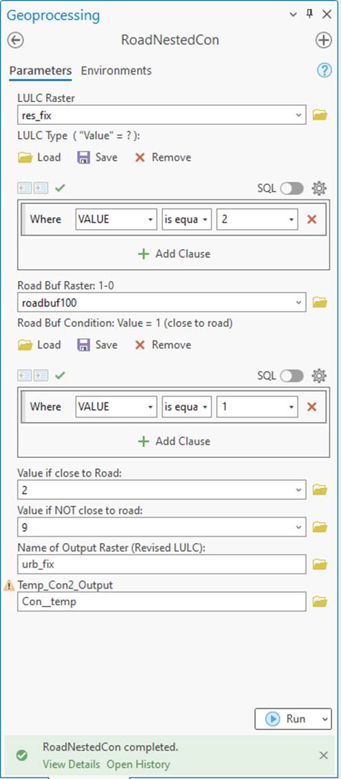
Residential, Urban, Rock: Click the small arrow next to the NestedConModels toolbox. We will start by using the “RoadNestedCon” model to deal with the confusion between the residential, urban and rocks classes. This model is based on the idea that areas that are really residential or urban are probably within 100m of a road. On the other hand, any areas that were classified as residential, urban or rock that are NOT within 100m of a road should probably be in the rock category. So here is what we will do:

Table 4: Rules related to roads:

Starting LULC class=>	Residential	Urban	Rocks
Close to road	Keep as Res.	Keep as Urban	Reclass to Urban
NOT close to road	Reclass to Rock	Reclass to Rock	Keep as Rock

See table 2 above for the class numbers that correspond to each of these classes.

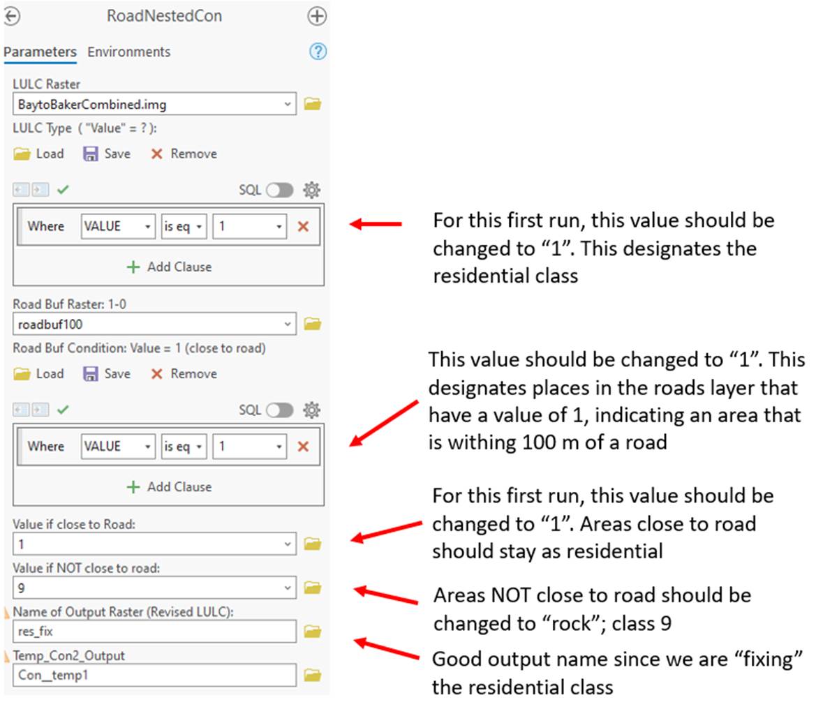
To achieve these reclassifications, we will run the “RoadNestedCon” model three times, once for each of our three starting – and problematic – LULC classes. To run the model, simply double-click on it. This brings up the following dialog box:

You will need to fill in several items in this dialog:

LULC Raster: This is the input for the model. Click on the drop-down tab and select your LULC layer. For your first model run, this is the “combined classes map” that you have developed. In the screenshot above, I’ve already filled mine in as “BaytoBakerCombined.img.” Note that for your second model run (for the urban class) the input file you enter here should be the output from the first model run. Similarly, the input for your third model run is the output from the second model run.

LULC type: This is the LULC class for which you are running the model. Start with the residential class which should be class 1. So, in the LULC type window, click on the 999 and enter the value 1.

Road Buf Raster: This should be “roadbuf100.” If it isn’t, click on the drop-down tab and select it.

Road Buf Condition: This is the value in the “roadbuf100” layer that designates areas that are within 100m of a road. Click on the 999 and replace it with a 1. Note that this is NOT an “optional” parameter! You will keep this condition as 1 for all three of the iterations of this model.

Value if close to Road: In your new LULC map that will be produced by this model, what LULC value do you want to use for residential areas that are close to roads? Based on Table 4 above, you want these areas to remain as residential so you want these to have an LULC code of 1. Replace the 999 with a 1.

Value if NOT close to road: Based on Table 4 and Table 2, what LULC code should you fill in here?

Name of Output Raster: (Revised LULC): Specify an output folder and output file name. You are going to be producing a whole bunch of these (at least 9 files) so I’d strongly suggest that you create a subfolder within your working directory to hold them; maybe a folder called something like “arcmodelout”. A good output file name for this first run might be something like “res_fix” since we are sort of fixing the residential LULC class……or you could just call is something like “output1.”

Temporary_Con2_Output: This should already be filled in to direct the temporary output to C:/Temp/temp. You can specify some other location if you want, HOWEVER it is important that there are no spaces in the pathname or file name (e.g., something like “C:/My Documents/temp” IS NOT OK). Note: each time you run this model, you will need to provide a new name for this output file. Unfortunately, it will not be overwritten on subsequent model runs. If you don’t change the filename, you will get an error message indicating that this file already exists and the model will not run. One easy solution is to simply increment the name; that is, “con_temp1”, “con_temp2”, “con_temp3….”

Run the model: After filling in each of these items, click OK to run the model. A small window will open to keep you informed of the progress of the model. When it has finished running, close this progress window and view the results. If you ran it correctly, you should see that the areas above treeline that were originally mapped as residential have been recoded to the rock class. Similarly, the exposed gravel bars along the Nooksack that were previously mapped as residential should now appear as rock. Finally, the residential areas around Bellingham should still be mapped as residential.

Check your result: When the model finishes, you will have two more layers available. One is the temporary file which you can delete by left-clicking on it and selecting “Remove.” The second is your output raster file. Unfortunately, Arc just assigns a random color scheme to it and there are no labels. To check your result, zoom in on the Mt. Baker area using scroll wheel on your mouse. Your screen should look something like this, though your colors may be different:

Ensure your topmost layer (layer on highest up on Contents bar) is the res_fix file (or whatever you named your new output from the RoadNestedCon. Press the Map tab on the ribbon and then click Explore. You can click around and see the effects of your conditional model.

In this case, my model output raster is called resfix. Rocks are class 9 and residential is class 1. You can check your work by using the explore button to click on areas that are given a residential classification versus areas with rock classification. All residential pixels that are not within 100m of a road should have been reclassified to the rock class. You can check and uncheck each layer to visually confirm this as well. Now let’s move on.

Now run the model again, this time for the urban LULC class. This time, the input LULC raster should be the output from the previous run (the run that “fixed” the residential class). The LULC type and Value if close to road should be changed to a value of 2 (designating urban). You will also need to specify a different output file name. Then click OK to run the model. Inspect the model output to confirm that you obtained the desired result.

Now run the model a third time, this time for the rock class. Make the appropriate changes to the input parameters and view the output to confirm that you obtained the desired results.

Water and Shadow:

FIRST: Ensure that your bbay_slope.img file has been added to the map via the add data button.

Recall that some areas that were in shadow on steep north-facing slopes were incorrectly mapped as water. We can address this problem using the SlopeNestedCon model. Navigate to the Catalog tab (on the bottom left hand bar). Double-click on the model to open this dialog box:

LULC Raster: This is the output from your final run of the road model (the run that focused on the rock class).

LULC type: Specify the water class (class 8 in my map).

Value if Slope is 0: These areas should be retained in the water class (Class 8 in my map).

Value if Slope is NOT 0: This will be a new LULC class that represents shadow. Call it class 12 (I used class 14 for clouds).

Name of Output Raster (Revised LULC): This is your new LULC map. Specify the location of your workspace and come up with a new filename.

Temp_Con2_Output: As with the first model, this is a temporary output file. You may need to change this if the file already exists.

Click OK to run the model. When it finishes, close the progress window and view the result. Is it what you expected?

Pasture, Crops, Clearcuts, Alpine: This is a big one and will require four model runs. The basic idea here is to use elevation to help separate these classes. Agriculture (Pasture and Crops) is something that only takes place at lower elevations (say below 200m). Forestry only takes place at intermediate elevations (say between 200 and 1500m). The alpine zone only occurs in – you guessed it -- areas above treeline (say 1500m). So our recoding should follow something like this:

Table 5: Rules related to Elevation:

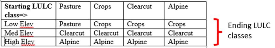
Again, refer to Table 2 above to confirm the class numbers that correspond to each class name.

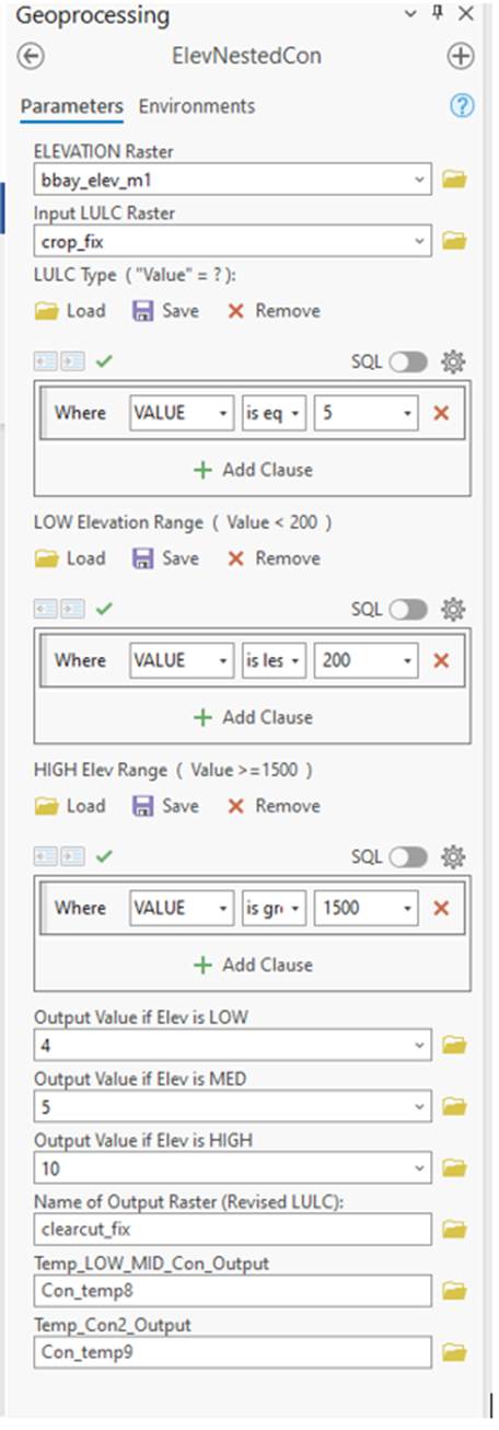
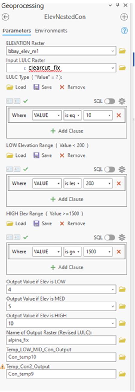
We can do this recoding by running the ElevNestedCon model. You will need to run this model four times; once for each of the LULC classes in Table 5. Double-clicking on this model brings up the following dialog box:

Note : Be sure to use the elevation grid (bbay_elevm1) with this model, not the .img version (bbay_elev_m.img). Either one SHOULD work but for some reason only the bbay_elevm1 version seems to work. As noted earlier, for those of you who are not Arc-savy, you will note that “bbay_elev_m1” will look like a folder in Windows Explorer. Go ahead and grab this entire folder along with the “info” folder and place BOTH of these in your working directory. I have also edited the ElevNestedCon model a bit so that you have to specify the ELEVATION Raster. This will be the “bbay_elev_m1” grid that you just copied. Then follow the directions below.

ELEVATION Raster: This will be the “bbay_elev_m1” grid that you just copied.

Input LULC Raster: For your first run of this model, the input LULC raster is the output from running the SlopeNestedCon model. In each subsequent model run, the input LULC raster is the output from the previous run of the ElevNestedCon model.

LULC Type: For your first run of this model, this would be the LULC code for Pasture; in my case, this is 3. In each subsequent run, it would be the next LULC class code from Table 5.

LOW Elevation Range: The default low elevation cutoff is set to 200m. You can use this or change it to a value that you feel is better.

HIGH Elevation Range: The default high elevation cutoff is set to 1500m. You can use this or change it to a value that you feel is better.

Output Value if Elev is LOW: Insert the appropriate LULC code that corresponds to the LULC class given in Table 5.

Output Value if Elev is MED: Note that this is NOT optional. Insert the appropriate LULC code that corresponds to the LULC class given in Table 5.

Output Value if Elev is HIGH: Insert the appropriate LULC code that corresponds to the LULC class given in Table 5.

Name of Output Raster (Revised LULC): This is your new LULC map. Specify the location of your workspace and come up with a new filename.

Temp_LOW_MID_Con_Output: This is a temporary file. You may need to change (increment) this filename with each model run.

Temp_Con2_Output: This is another temporary output file. You may need to change (increment) this filename with each model run.

Fill in each parameter and click OK to run the model. When it finishes, close the progress window and view the result. Is it what you expected? After running this model for the alpine class (your sixth run of this model) you should have a pretty good map.

Moving your Final Map back to ENVI: After your fourth run of the ElevNestedCon model, right-click on this final layer and go to Data-Export Data

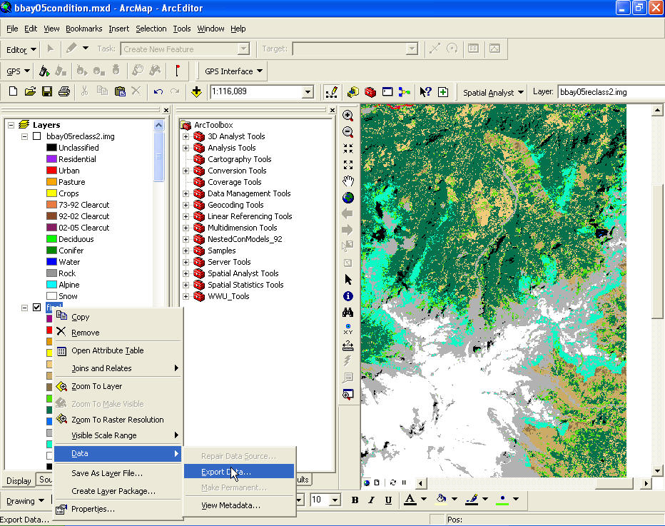
The Export Raster Data dialog box will appear. Specify a location and filename and specify an output format of “ENVI”. .

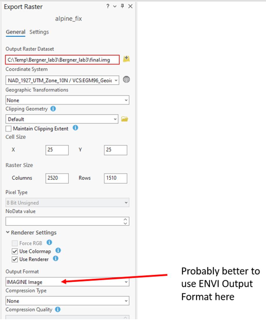
Before you save, make sure you have a good file path for your output raster.

You MUST save this file as a .img (IMAGINE) file for it to open back up in ENVI. Also, you have to check the “Use Render” and “Use Colormap” buttons.

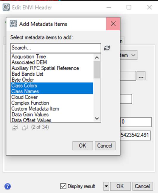
Open the file in ENVI. In order get it to display properly in ENVI, you will need to edit the metadata. To do so, right-click on the file and go to View Metadata, then to Edit Metadata. In the Edit ENVI Header dialog box, click on and select Class Names and Class colors and Number of Classes (and the number of classes should be 13; 0-12 with 0 being “unclassified” and 12 being your new “shadow” class). However, you will probably find that Class 0 is really residential and class 11 will probably be shadow.

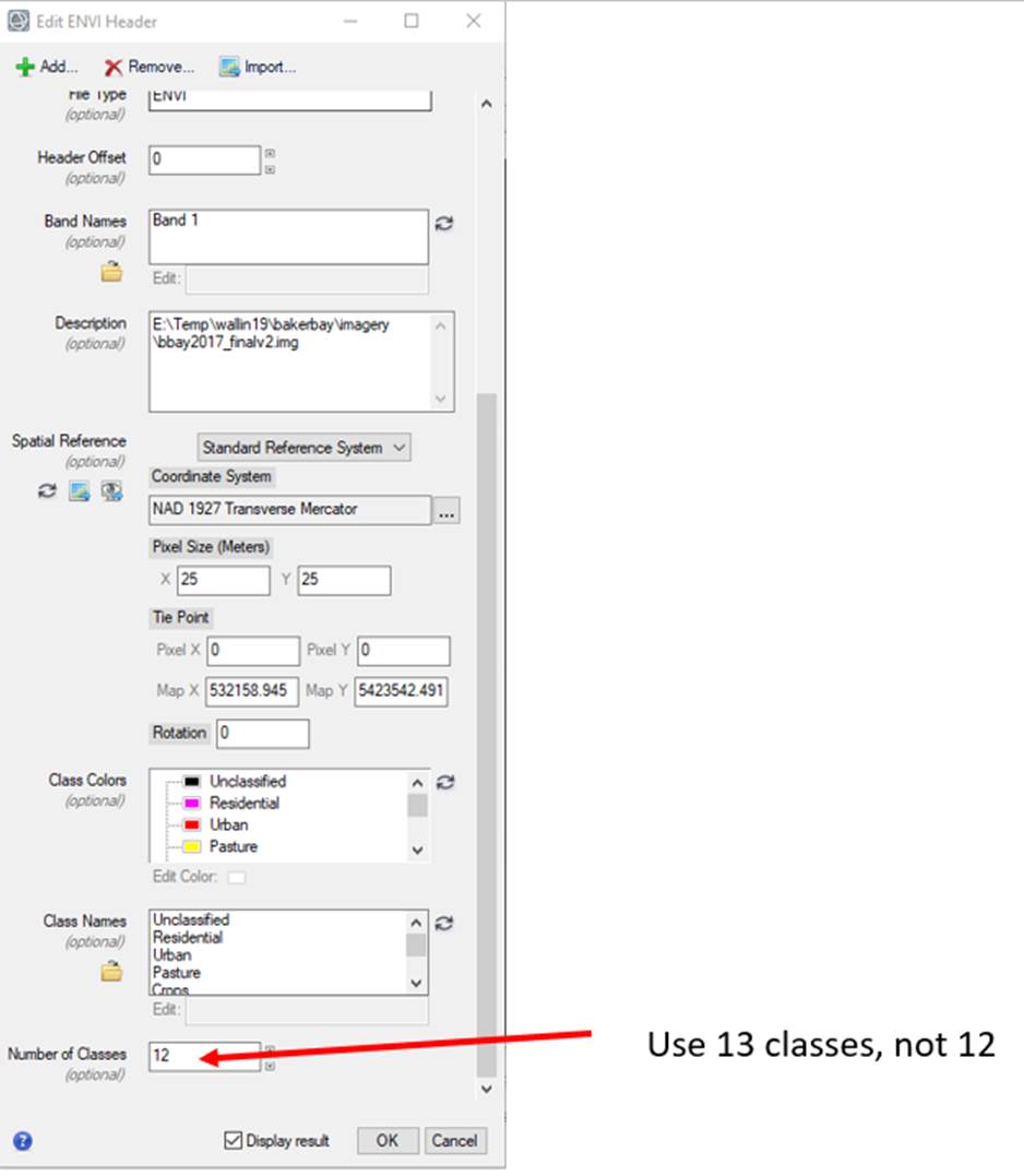
Your classes will be listed from 0-12. You will rename these classes in order. Residential will now be 1, urban 2, and so on. Edit the class colors to match the ROIs. Your last class (class 11 or maybe 12?) will be your shadow class.

You can now edit the class name and color for Class 12 (your shadow class). You can compare this image to your original combined classes image to see if you obtained the result that you wanted, then move on the Classification Accuracy step.Converting from an ENVI Standard file to an ENVI Classification: Back in ENVI, go to your Available Bands List-File-Open Image File and get the ENVI file that you just created in ArcMap. You can load this into a display and it will come up as a gray-scale image. In order to restore the color scheme and run an accuracy assessment, you need to convert this ENVI Standard file to an ENVI Classification Image. The easiest way to do this is to go to the Available Bands List, right-click on the file and go to Edit Header. In the Header Info dialog box, change the File Type from ENVI Standard to ENVI Classification. After clicking OK, you will be asked to specify the number of classes in the image. In our case this is 13 (note that we started with 11 but we added a shadow class plus there is also an “unclassified” class, making a total of 13 classes). Click OK and this will bring up the Class Color Map Editing dialog box. Work through the classes, editing the names and colors to restore the same color scheme as the one you started working on in ArcMap. After doing this, you can compare the two image to confirm that you obtained the result you wanted.

Classification Accuracy: Now you can generate a new confusion matrix using this final ENVI Classification image. Use the same test2019QC_11class.roi file that you used previously. Refer to the instructions above for guidance. After generating the revised confusion matrix, pull it into Excel and rearrange it as you did previously. You should see some improvement in your classification accuracy but it will probably on the order of 5% or so. Quantitatively, this may not seem like much. However, visual inspection of the image will reveal significant improvement; among other things, the residential and urban areas above treeline on Mt. Baker will now be gone.

Step 8: Lab Report. Write a lab report. Tell us which spectral classes (and how many) you combined to form each information class and why. Are some information classes more variable than others? Why? Do you think some of your information classes could be further subdivided with some additional work? What additional information might you need to do this? How many information classes did you end up with? Include all the necessary images and tables. How much area is in each information class?

Several people have expressed confusion about what should be included in your lab report. This lab has involved quite a bit of work and it will need to be somewhat longer than the lab reports you have written earlier in the quarter. Your classification was really done in two stages and you should summarize your methods, results and implications/conclusions from each of these two stages. These stages were:

1. Assignment of spectral classes to information classes based on reference data. You split your reference data into a training set and a test set. You prepared a cross tabulation of your 50 spectral classes and your 11 reference classes and used this to objectively assign spectral classes to information classes. You then used your test set to do an accuracy assessment.

2. Finally, you used several conditional models in ArcMap to refine your map. This probably enabled you to improve your classification accuracy or at least achieve a similar classification accuracy while retaining more of your classes. Do an accuracy assessment of this map using the same test set that you used previously.

For each of these 2 approaches, your report should include:
a) your best map of the study area;
b) an accuracy assessment, probably at several levels (you started doing your accuracy assessment for 11 classes but may have decided to collapse your map down to perhaps 8 or 9 classes; how did the accuracy change as you did this?);
c) a table showing the % of the study area in each cover type.

As part of your discussion, you should describe how your results changed with each new approach. Are there any problems with your reference data that might be influencing your results? In addition you your quantitative accuracy assessment, you should also do a visual, subjective assessment. What were the obvious flaws at each stage? How and why did each stage of your analysis improve your result? What would your next step be if you wanted to refine this even further? 

---

---

Return to ESCI 442/542 Lab Page

Return to ESCI 442/542 Syllabus

Return to David Wallin's Home Page