|
Objectives: • NAIP imagery • Lidar derived DSM • Creation of Ground Truth data • Image segmentation • Supervised Image Classification • Accuracy Assessment
Tools: • ArcGIS Pro • Washington DNR Lidar Portal: https://lidarportal.dnr.wa.gov/
Data: None to download from Canvas
Submission: Lab report submitted to your TA
Supplemental: ArcGIS Pro documentation on:
|

Objective: You will be acquiring NAIP imagery of Western Washington University from 2013 via ESRI online service. You will be combining this 4 band data with lidar data downloaded from the DNR lidar Portland. Using the high resolution aerial data, you will be creating ground truth data for your own accuracy assessment. You will then segment your image and preform a supervised classification with 6 classes.
|
Class |
Code |
Color |
|
Water |
1 |
|
|
Grass / low vegetation |
2 |
|
|
Tree / tall vegetation |
3 |
|
|
Roads / low impermeable surfaces |
4 |
|
|
Buildings |
5 |
|
|
Shadows |
6 |
|
- Open up ArcGIS Pro and start a new map project. Remember to be very aware of the file directory where you are creating and saving data for your project. Make sure that you have a solid workflow for saving and backing up your work on some other drive other than the remotely accessed computer. U drive, OneDrive, Box, Google drive, etc.
- We want to import and copy NAIP data from 2013. We want 2013 data because we will also be using some lidar data and the most recent lidar data of the area was from 2013. We want our imagery to match the date of the lidar data.
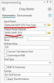
See below for instructions on importing NAIP imagery, and luckily, statewide Washington NAIP from 2013 is available in its own layer. Select “Statewide NAIP 2013 True Color” and bring it into ArcGIS Pro. A brief note about data on ArcGIS online… You will want to check the source of your data if using anything for publication. In this case, it is a user that has uploaded the data and we can take advantage of that, but we don’t know for certain that they didn’t do anything to the data before uploading to ArcGIS online. It is a good idea to try and stay with trusted sources, but for the purposes of this lab, we can use data someone else has made available to save us a few steps.
Click “Add Data” in the Map tab in ArcGIS. Select ArcGIS Online and type “Washington 2013 NAIP” in the search bar. Finally, select “Statewise NAIP 2013 True Color” and hit “OK” to add this to the map.
Check out the imagery and you can change the band combinations if you like. Make sure you have 4 bands of information (R,G,B,NIR).
NOTE (2/17/2025): If you
run into problems accessing the NAIP image, go the the student drive
Y:\Courses\ESCI Wallin (442)\ESCI442_w2025\
and go to the
“Imageseg” folder and get a copy of “wallin_naip2013.gdb” and move it to your
workspace on C:\temp. Open it using the “Add data” tab described above.
If
you go this route, you can skip to the section below that discusses loading the
lidar data.
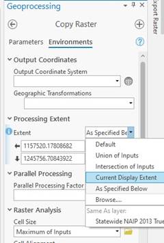
Zoom into WWU and get your window to display as close to this as possible and select the tool “Copy Raster” (Analysis → Tools → Copy Raster). We are going to use the extent of the display window to define the area of the raster we want to copy. Make sure to have water in the image.
Name your output WWU_2013 and leave the location in the.gdb. You MUST click on the Environments tab and define the Processing Extent as “Current Display Extent”. If you try and copy the raster and ArcGIS Pro just runs endlessly, you may have the Extent set wrong and effectively trying to copy the entire 2013 NAIP dataset.

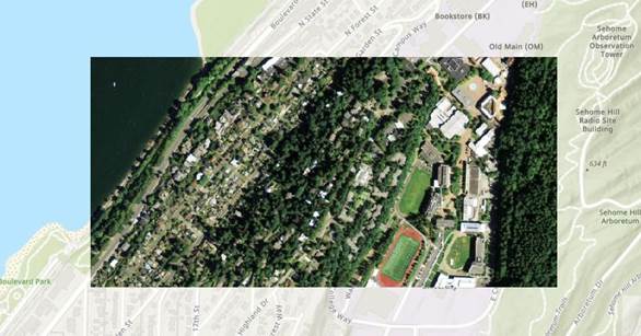
When you zoom out, you should have something like this:
Save your progress and we are going to go get some lidar data.
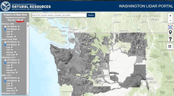
-Go to https://lidarportal.dnr.wa.gov/
Lidar data can be found for free for most states with a little digging. For Washington, The Department of Natural Resources has created this fantastic portal for all publicly available lidar data for the state of Washington.

You can take a moment to check out the website. To make
things easier to find the data we want, go ahead and click on “hide all” at the
top of the grey box so we can see the map underneath. Zoom to WWU. Use the pin
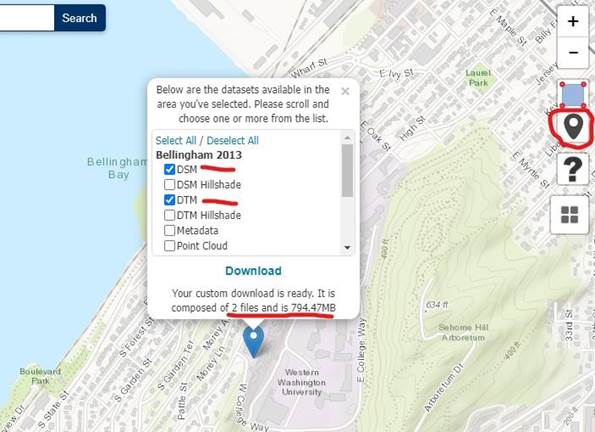
tool ![]() and drop a point in the approximate
center of where our imagery is located. You will be given the option to
download multiple different layers from different data sources.
and drop a point in the approximate
center of where our imagery is located. You will be given the option to
download multiple different layers from different data sources.
The best thing to do is to first click “Deselect All” and then select the Bellingham 2013 DSM and DTM. It should be 2 files that are 794.47MB in size. This is a large file that we will be clipping only a small portion from. You should delete the large files once we have what we are interested in.
-Unzip the files and drag and drop the Bellingham_2013_dtm_6.tif and the
Bellingham_2013_dsm_6.tif into ArcGIS Pro. Click yes if Arc asks to compute statistics for the layers. Check out the data. The difference between a DTM and a DSM is that a DTM is the Terrain with all buildings and vegetation removed. The DSM is the Surface derived from the lidar points.
Imagine just laying a sheet across the area and all the trees and buildings are holding up the sheet. We want to create a copy of the DSM and DTM for just the area of the NAIP imagery.
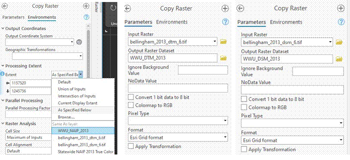
-Use Copy Raster TWICE. Once to copy the dtm and once to copy the dsm. IMPORTANT, you must set the Environments > Processing Extent to match your WWU_NAIP_2013 layer.
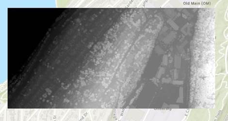
Once you have your copies, you don’t need to save the original zip file or the unzipped tiff files. Delete them if space is of concern. Your lidar outputs should look like this:

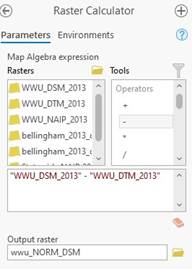
You can see the elevation of the hills and the location of all the buildings. All of the buildings values are elevation currently. This isn’t helpful for us to know the height of a building. We need to normalize the DSM so the Z values are height above ground and not elevation above sea level. The process of normalizing the data is very simple. Using the Raster calculator the equation is simply:
DSM - DTM= Normalized DSM
W
-Open the raster calculator and input the equation and name your output WWU_NORM_DSM
Your output should look like this:
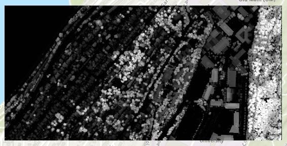
Element: The normalized lidar raster. Discuss how the normalized raster can aid in supervised classification.
This is the height of all the trees and buildings in the area. This is a raster image where the pixel values are NOT radiance values but are height. In this case, the values are from data we downloaded from a state agency, and they are unfortunately given in US feet. If you investigate the image, you will be able to find the tallest tree in the area or the tallest building.
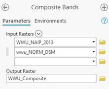
We now have data that will help our classification by distinguishing things that are spectrally similar, but have different heights (e.g., roads and buildings or trees and grass). We need to add this image as an additional band to our NAIP raster. This will create a new raster data set with 4 bands of spectral information and one band of height values. Ultimately, they are all just bands within a raster that contain digital numbers representing something.
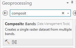
-Open the Composite Bands tool and create a new raster comprised of the NAIP imagery and the lidar data. This is what we will be working with for the rest of the lab.

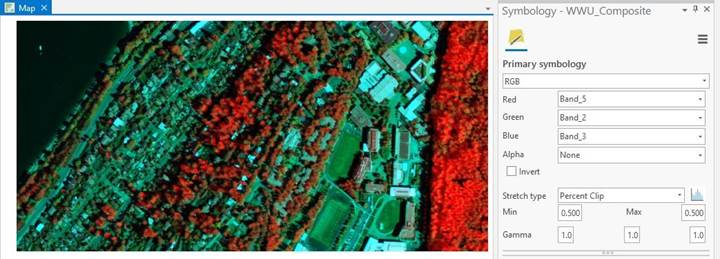
Take a moment to check out the different ways for symbology with the new composite raster. If you put band 5 in the red channel…. Tall things will turn red. This is different from putting the NIR band in the red channel. With the lidar data, tall things are more red than short things.

-Once you are done investigating the symbology, change your image back to “true color”. We are going to now make ground truth data for our area using the NAIP imagery. Create a new feature class with Geometry Type “Point” and a coordinate system to match the current map. It should automatically be added to your map.
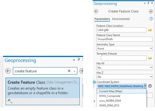
-Hit Run, then….
-We need to add two fields to the newly created GroundTruth data. “GrndTruth” and
“Classified”. The spelling matters.
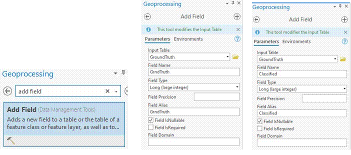
In the “Contents” pane, open the attribute table for GroundTruth by right-clicking on it…
When you open the attribute table for Ground Truth you should see this:
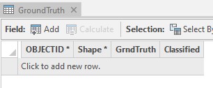
We are going to add points to GroundTruth and add a value to the GrndTruth column that corresponds to our class codes.
|
Class |
Code |
Color |
|
Water |
1 |
|
|
Grass / low vegetation |
2 |
|
|
Tree / tall vegetation |
3 |
|
|
Roads / low impermeable surfaces |
4 |
|
|
Buildings |
5 |
|
|
Shadows |
6 |
|
-In the edit tab, select create and then GroundTruth and points.
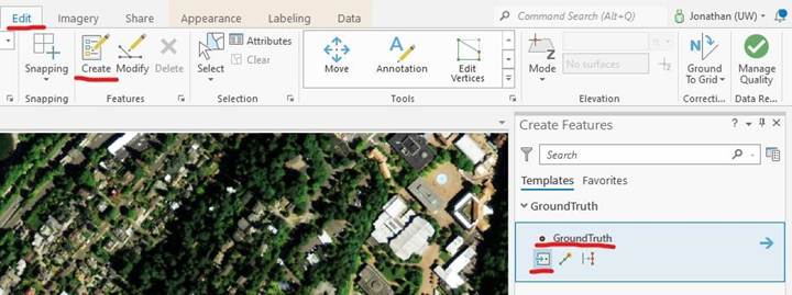
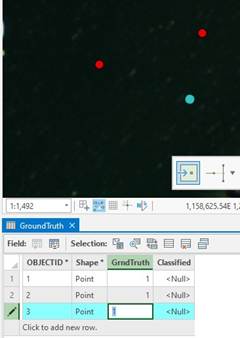
 -Add points by clicking on the map. This
will add new rows in
the attribute table and with each new addition, fill in the GrndTruth value with the appropriate class code. Create between 20 to 40 points for each class above. Make sure to collect samples across the entire image. When you are done, you should have ~200 points.
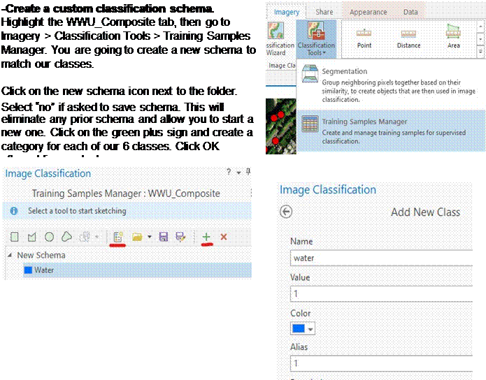
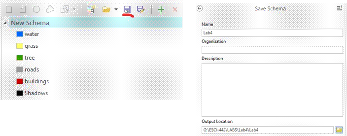
Save the schema in a location you can find and name
it WWU_Schema
-Classification Tools. With your WWU_Composite layer selected, click on the Classification Tools and Select Segmentation. For starters, we’ll segment the image and then we will move on to classifications
For this lab, it is important that you experiment with the values that produce the segmentation and the different classifiers. You should understand what each does and be able to provide a description of how the classifier works in the lab write up. This will require you to do some research on your own.
-Segmentation.
“Segmentation is a key component of the object-based classification workflow. This process groups neighboring pixels together that are similar in color and have certain shape characteristics. In addition, you can use the Show Segmented Boundaries Only option if you want to display the segments as polygons with the source image visible underneath.
After you run segmentation, you will want to see the underlying imagery to verify that the objects make sense. Press the L key to toggle on and off the transparency of the segmented image. The preview is closest to the output result when you zoom in to source resolution and make sure the display is large enough.” https://pro.arcgis.com/en/pro-app/latest/help/analysis/image-analyst/segmentation.htm
For image segmentation there are three setting: Spectral detail, Spatial detail, and Minimum segment size.
Spectral Detail
Set the level of importance given to the spectral/elevation differences of features in your imagery. In our case, in addition to the four spectral bands (Blue, Green, Red, NIR) we have that 5th band that represents height above the ground (units are feet, not meters; yuck!). This elevation data will be treated in the same way as the spectral data.
Valid values range from 1.0 to 20.0. A higher value is appropriate when you have features you want to classify separately but have somewhat similar spectral characteristics. Smaller values result in more smoothing and longer processing times. For example, a higher spectral detail value in a forested scene will result in greater discrimination between the different tree species.
Spatial Detail
Set the level of importance given to the proximity between features in your imagery.
Valid values range from 1 to 20. A higher value is appropriate for a scene where your features of interest are small and clustered together. Smaller values create spatially smoother outputs. For example, in an urban scene, you could classify impervious surface features using a smaller spatial detail value, or you could classify buildings and roads as separate classes using a higher spatial detail value.
Minimum Segment Size
This parameter is directly related to your minimum mapping unit. Segments smaller than this size are merged with their best fitting neighbor segment.
Reading the description of each setting you need to consider how spectrally similar our classes are, how spatially complex they are, and the size of the classes we want to segment compared to our image resolution.
We have 6 broad categories, so they are not that spectrally similar, but we do want to separate out buildings from roads. Our image resolution is only 1m so consider how big our smallest classes are and how many pixels do you think will be present.
There isn’t one correct answer to what values you select. You can start with the defaults and then hit the Preview button. You can then change the parameters and the image will be resegmented. As a general rule, too many segments are better than not enough. The only issue is that the computation is more intense with a lot of smaller segments. A check you can do is to zoom in on some houses with just the segment boundaries showing . In the example below, the house is included in the same segment as a road. This is bad. This was fixed by turning up the spectral detail until the house is segmented out from the road.
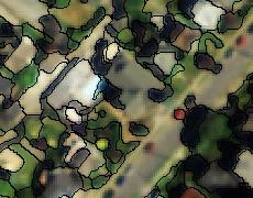
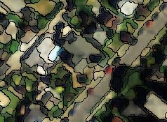
When you have values for your segmentation that you like, specify an output dataset folder and a file name and click Run.
Element: You will want to note your segmentation values you used AND justify why you used them. Discuss what changing the values actually does and not just justify your values because “it looked best”.
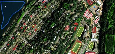 -Training Samples Manager. Click on your WWU_Composite image in your
Contents pane. Then go to Classification
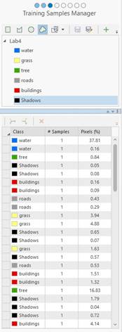
-Training sample manager. Click on
the folder icon
 ![]() and Browse to an existing schema
and load the scheme that you have already created. You will now be drawing polygons around features and
telling the computer what each polygon is. You can use any of the polygon types
and select a class and draw a polygon onto the image. Spend a good amount of
time on this and zoom in when creating the polygons. Make selections across the
entire image. Try your best to not create a polygon with two different classes
in it. Shadows can be tricky because they are inherently at least two classes.
Because we are making shadows its own class, a tree in shadow becomes the
shadow class and is no longer a tree as far as we are concerned. Also, when creating training polygons, try NOT to create a
polygon that includes one or more of your ground truth points. If, for example,
ALL of your ground truth points for grass are included in your training
polygons for grass, your producer’s accuracy for this class will probably be
100% and this may be an unrealistically high indication of the “true”
producer’s accuracy. When you are happy with your training samples,
click on the Save Training Samples icon,
and Browse to an existing schema
and load the scheme that you have already created. You will now be drawing polygons around features and
telling the computer what each polygon is. You can use any of the polygon types
and select a class and draw a polygon onto the image. Spend a good amount of
time on this and zoom in when creating the polygons. Make selections across the
entire image. Try your best to not create a polygon with two different classes
in it. Shadows can be tricky because they are inherently at least two classes.
Because we are making shadows its own class, a tree in shadow becomes the
shadow class and is no longer a tree as far as we are concerned. Also, when creating training polygons, try NOT to create a
polygon that includes one or more of your ground truth points. If, for example,
ALL of your ground truth points for grass are included in your training
polygons for grass, your producer’s accuracy for this class will probably be
100% and this may be an unrealistically high indication of the “true”
producer’s accuracy. When you are happy with your training samples,
click on the Save Training Samples icon, ![]() then save to your geodatabase (in my case,
WWUseg.gdb). You will then need to hit refresh in your .gdb for your training
data file to show up in your gdb file. You may have to come back to
refine your classes later if needed.
then save to your geodatabase (in my case,
WWUseg.gdb). You will then need to hit refresh in your .gdb for your training
data file to show up in your gdb file. You may have to come back to
refine your classes later if needed.

-Train. Read up on the classifiers here: https://pro.arcgis.com/en/pro-app/latest/help/analysis/image-analyst/classify.htm
Click on your WWU_Composite image to highlight it. Then go
to Imagery-Classification Tools-Classify
For our supervised classification there are three options:
• Maximum Likelihood—The maximum likelihood classifier is a traditional technique for image classification. It is based on two principles: the pixels in each class sample in the multidimensional space are normally distributed, and Bayes' theorem of decision-making.
• Random Trees—The random trees classifier is a powerful technique for image classification that is resistant to overfitting and can work with segmented images and other ancillary raster datasets. For standard image inputs, the tool accepts multiband imagery with any bit depth, and it will perform the random trees classification on a pixel basis, based on the input training feature file.
• Support Vector Machine (SVM)—The SVM classifier provides a powerful, supervised classification method that can process a segmented raster input or a standard image. It is less susceptible to noise, correlated bands, and an unbalanced number or size of training sites within each class. This is a classification method that is widely used among researchers.
There is once again no one correct option. Pick one, then add your training data and your segmented image. After doing so, you will have the option to specify which Segment Attributes to include. Not sure what “Active chromaticity color” but be sure to include “Mean digital number” and “standard deviation.” Your choice on whether to include the others. “Count of pixels” just involves using the size of the segment as a variable. “Compactness” is just that; is the segment compact or long and skinny. “Rectangularity” might be interesting to try since our scene includes buildings.
Finding the best combination will take time. Refer back to the ESRI documentation. Your goal should be something that looks even better than this. The classification above has lots of shadow misclassified as water. The one below looks better.
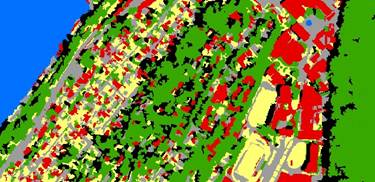
Element: When you find a combination that works well for your image. Record the classifier and values you used. You must also provide a description of how the classifier worked. You can start your research on the ESRI website but a description of how the classifier functions is required. A conceptual diagram may be helpful.
The previous step was to view previews and test out value
combinations. This step will actually run the full classifier and output your
classified image.
-Accuracy
Assessment. Go to Analysis-Tools,
which brings up the Geoprocessing dialog. Search for “Accuracy Assessment” and
select the “Update Accuracy Assessment Points” tool.
This step refers back to your initial ground truth data you created. You should have around 200 points in your ground truth data.
We are using points for our accuracy assessment, but we could potentially be using polygons. If we were using polygons, ArcGIS would create random points inside the polygons and then follow either a totally random distribution of the points, or distribute the points based on the area of the polygons for each class. That is why there are different options in this step. Save your data before continuing, as this step likes to crash ArcGIS.
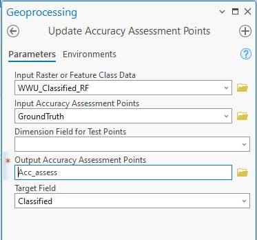
In the “Update Accuracy Assessment Points”, enter:
-The Input Raster is the result image resulting from running your classification.
-Input Accuracy Assessment Points is your “GroundTruth” layer containing the set of points you selected earlier.
-Leave the “Dimension Field for Test Points” blank
-Select a name for the Output Accuracy Assessment Points
-Target Field: Classified.
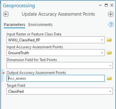
Click Run
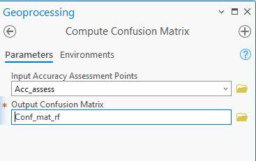
Generate a Confusion Matrix: Go back to the Geoprocessing dialog and search for and open the “Compute Confusion Matrix” tool.
-Input Accuracy Assessment Points is the output from the previous tool
-Select a name for the Output Confusion Matrix
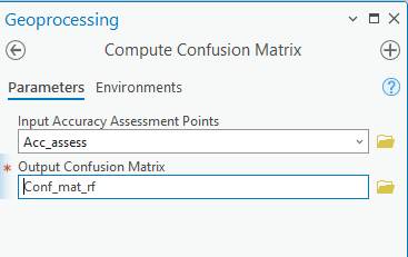
Click Run.
When finished, the Confusion matrix will appear at the bottom of your Contents pane. Right-click and open it.
If ArcGIS crashes, you should be able tor recover your Confusion Matrix. Go to Catalog → Databases → Confusion Matrix and drag and drop this into the map.
Element: Include a copy of your confusion matrix
-Reclassifier. You can potentially use this step to remove any water that was on land or other misclassified segments. It is optional and likely unnecessary. You can click run, but if you have nothing selected, the reclassified image will be identical to the original classified image.
If the program crashed, highlight your Preview_Classified layer that you chose for the classification. Go to Imagery → Classification Tools → Reclassifer
Element: Include a copy of your final classified image with legend.
Done!
The steps in the lab are relatively simple. You will need to dig deeper for information about the algorithms used for the supervised classification for your report. You might want to try running both the Random Forest and the SVM classification methods. This is optional.