ESCI497Z:
UAS for Environmental Research and Monitoring
Image
Segmentation of UAS Imagery
Objective:
The
objective of this exercise is to explore the use of a new software package to
conduct a segmentation and classification of a portion of our Glacier Springs
image.
Introduction:
When
using moderate resolution imagery (such as LANDSAT imagery with a pixel size of
30 m), pixel-based classification works quite well. Pixel-based classification
involves classifying each pixel based solely on its spectral properties without
considering the characteristics of any of the surrounding pixel. With very high resolution (VHR) imagery (pixel size of ~1 m down to a
few centimeters), pixel-based classification does not work. Instead, the
emerging consensus is to perform image segmentation as a pre-processing step
prior to classification. Image segmentation involve joining adjacent pixels
with similar spectral properties into “image segments.” The image segments can
be of irregular shape and size. Image segments are then classified on the basis of the mean and variance of the spectral
properties of the pixels in each image segment. The spatial properties (shape
and size) of each image segment can also be used as
part of the classification process.
For today’s lab we will use a
variety of software packages to carry out both the image segmentation and
classification processes.
Data:
The
image was acquired on Sept 28, 2016 using our 3DR Solo
quadcopter carrying a Canon S100 camera that has been modified to cover the
near IR portion of the spectrum. The full image is available here:
J:\Saldata\ESCI-497\glacier_sp. This
folder includes both a “red edge” version of the image (that will be our
primary focus) and a true color version (acquired on Sept 18) that will be
useful for interpretation. The GCPs for this area were in the State Plane
coordinate system with coordinates in units of feet (ug!!!) so the pixel size for both images in 0.1 feet. Weird
units, I know.
I’ve
clipped a small subset from this larger Glacier Springs image and I’ve
converted it to UTM coordinates. The pixel size for this image is 3 cm. This is the image that we will be using for our analysis.
This image (rededge_ndi2_utm.tif) includes 4 bands (aka
“layers”). Bands 1, 2, 3 are the red edge, green and blue, respectively. Band 4
is a “normalized difference index” that was calculated
using:
NDI
= (red edge – blue)/(red edge + blue)
This is an index to photosynthetic rate. More about
this later.
Go ahead and move this entire
J:\Saldata\ESCI-497\glacier_sp folder to your workspace on C:\temp I my case, I
will be working on C:\temp\wallin
.
Image
Segmentation with Montiverdi and the Orfeo Toolbox:
This is an open source image
processing package. I’m still on the steep end
of the learning curve with this package but it seems to have some nice
features. So here goes….
Open Montiverdi, Then go to File-Open
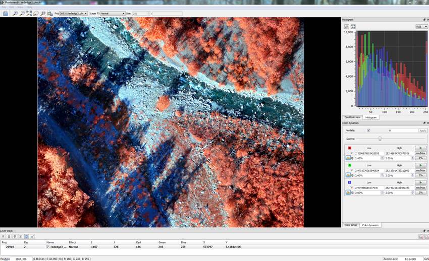
Images. Open your red edge subset image. It should look like this:
Image
segmentation with the Orfeo Toolbox (OTB):
Go to View-OTB
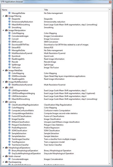
Application Browser. This brings up a window with a bunch of options. Scroll
down until you see the options for the “Large-scale Mean-shift Segmentation
(LSMSS):
Here is a link with some additional information about
the steps that we will be running: https://www.orfeo-toolbox.org/CookBook/recipes/improc.html#large-scale-mean-shift-lsms-segmentation
And
here is a link to the paper that is referenced above Michel_et_al_2015_Stable_Mean_Shift_algorithm
And
here is another paper that I found to be quite useful:
Chehata_etal_2014_Object-based
change detection using high-resolution multispectral images.pdf
The
Mean-Shift Segmentation Algorithm:
Briefly, the MSS algorithm works by searching for
local modes in the joint feature (spectral) and spatial domains. In geek-speak,
the algorithm “searches for local modes in the joint feature and spatial domain
of n+2 dimensions, where n is the number of features (spectral
bands) that are added to the two spatial dimensions.” So, just like ISODATA,
LSMS is identifying pixels that are close together in spectral space but
ALSO close together in geographic space; the spatial dimensions. There are two parameters that control the segmentation
process. The spatial radius controls
distance (number of pixels) that is considered when
grouping pixels into image segments. The range
radius refers to the degree of spectral variability (distance in the n-dimensions of spectral space) that
will be permitted in a given image segment. The range radius should be higher than the maximum spectral difference
between intra-segment pixel pairs and lower than the spectral difference
between segment pixels and the surrounding pixels outside the segment. The spatial radius should be close to the
size of the objects of interest (Chehata et al. 2014).
I’ve
done a whole bunch of segmentations with a different image (centimeter
resolution image acquired from an unmanned aircraft) using a range of
parameters. Just to give you a feel for the different results, here are some
examples (subset of our full scene) using different combinations of spatial radius and range radius. In each of the four examples below, I used a minimum
region size of 500 pixels (about 0.5 m^2).
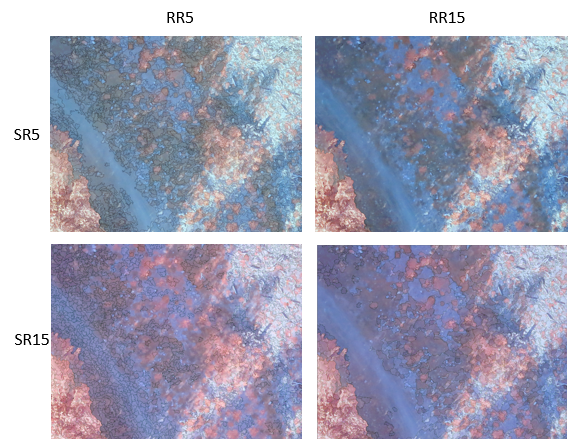
Note that as the SR and RR increase, the resulting
image segments get larger and seem to include scene components that are
obviously quite different (eg, vegetation and rock).
After experimenting quite a bit, I found that I was not able to obtain “clean”
image segments until getting down to SR: 2 and RR: 4.
Parameter selection in this segmentation step is
critical. If the segments are too large, dissimilar objects are included within
each segment and withi-segment variability
compromises the classification accuracy. If the segments are too small, individual
objects in the scene (e.g. a single building or a
single tree canopy) will be subdivided into separate image segments and the
spatial properties of these objects will be lost. Methods for optimizing
parameter selection are under development in the literature. At present, parameter
selection is mostly done using trial and error. Here
is one paper that presents a possible approach to optimize parameter selection.
((link to Ming paper)).
For today’s lab I’ve just
taken a wild guess at parameter selection.
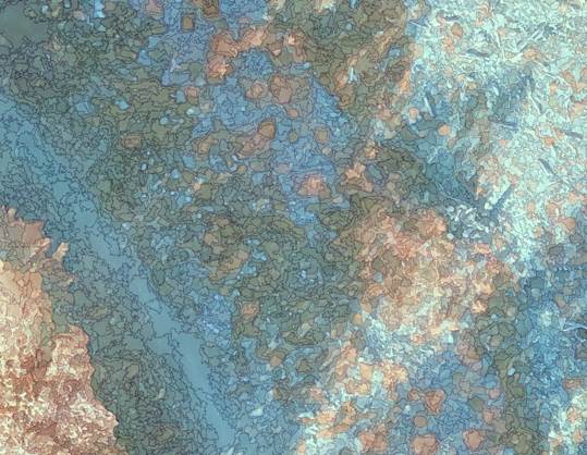
Go ahead and perform a segmentation (the 4 steps that
follow) using SR: 2 and RR: 4 and a Minimum Regions of
500.
Step
1: Large-Scale Mean-Shift Smoothing (LSMSS)
Let’s
start with Step 1. Read the documentation, then specify
your input image (the red edge subset) and filenames for the “Filtered output”
and the “Spatial Image.” (be sure to give each of these output files a .tif suffix) I’d strongly
recommend that you put all of your output files in a separate folder. I called
mine “segout.”
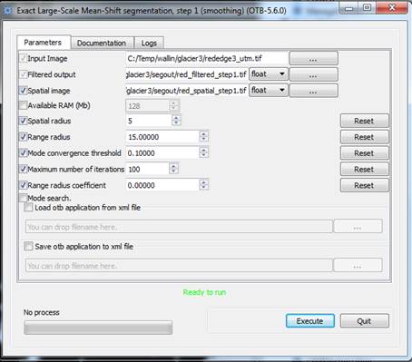
Take all of the default parameters EXCEPT, you should
uncheck the Mode Search option.
.Execute.
Run
Step 2: LSMSSegmentation
Use the “Filtered output” and the “Spatial Image” from
Step 1 as input files for Step 2. Specify an output image (with a .tif suffix). Don’t set a Min
Region Size. If you set a Min Region size here, these small regions will be
set to the background label and will not be subject to further processing. This
would lead to “holes” in your final output. We’ll deal
with these small regions in a different way in the next step. Specify a Directory for temporary fields. This
can be your segout folder. These temporary files are automatically deleted at the end of this step.
Click Execute
but be patient. It appears that nothing is happening but all is well.
When this step finishes, your red_step2.tif will be displayed. Mine looks like this:
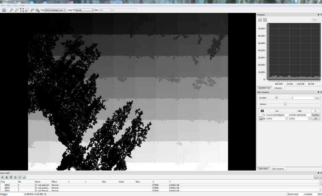
The blocky nature of this image is just an artifact of
the way that the image segments are labeled at this
point and the fact that the segmentation proceeds in “tiles” or subsets of the
full image. This means that each of the segments in a given tile are labeled sequentially. The labeling starts with the image
segments in the upper left tile (low label numbers; darker shading) and the
labels for the segments in the lower right get higher label numbers and hence
lighter shading. This issue will be addressed in later
steps.
Run
Step 3: LSMSSmall Regions Merging Application
This step can be used to
filter out small segments. Segments below the threshold size are
merged with the closest big enough adjacent region based on radiometry.
The “Input image” is your original red edge subset.
The “segmented image” is the output from step 2. Specify an output image with a
.tif suffix.
Let’s
go with a Minimum Region Size of 500. With
3 cm pixels, a region composed of 500 pixels would have an area of about 0.5 m^2.
Click Execute and again be patient. It is not clear that
processing is underway but it is.
Step
4: LSMSS Vectorization
This step produces a vector output of the segmented
image. The output is a shapefile that with a polygon that delineates each image
segment. For each image segment, the attributed file provides the mean and
variance of the brightness value for each band for all pixels in the segment
and the number of pixels in each segment.
Again, the “Input image” is your original red edge
subset. The “Segmented Image” is the output from step 3. The output file is a
vector file and it must have a .shp suffix.
Again, click Execute
and be patient.
Examine
your Image Segmentation Result in Arc
Open ArcMap and use the ![]() button to add both your original image
(rededge_ndi2_utm.tif) and the shapefile that you created in Step 4 in OTB (mine
is called rendi_step4_min500.shp). Turn both on. If
you have the shapefile on top, you can right-click and go to Properties-Display and set the
transparency to 50% so you can “see through” the shapefile to see the image
below.
button to add both your original image
(rededge_ndi2_utm.tif) and the shapefile that you created in Step 4 in OTB (mine
is called rendi_step4_min500.shp). Turn both on. If
you have the shapefile on top, you can right-click and go to Properties-Display and set the
transparency to 50% so you can “see through” the shapefile to see the image
below.
From the Table
of Contents, right-click on your shapefile and Open the Attribute Table. The first part of mine looks like this.
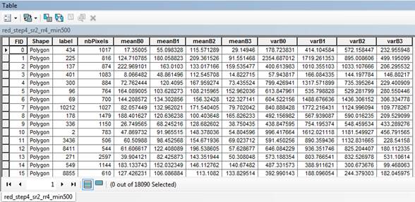
Each row in the table represents one image segment. So
note that in my case, my segmentation consists of 18,090 image segments. The
fields in this table are:
FID: is just a segment ID#.
Shape: all are polygons
Label: I have no idea what this is??
nbPixels:
the # of pixels in the image segment
meanB0,.., B3: mean value in
band 0 (red), 1 (green), 2 (blue), 3 (NDI) for all of the pixels in this image
segment
varB0,.., B3: variance of the
values in B0,..,B3 for all of the pixels in this image segment
All of the information in your attribute table is saved in a .dbf file with the same prefix as your
shapefile. Open the .dbf file in Excel and save a copy as an Excel file. For
some reason, the FID does not get saved as part of the
dbf file. So in the Excel file, you will need to
insert a column, label it “ID” and insert segment id# starting with 0. Also, very
important, delete the “Label” column!!!!!
So now, we want to identify groups of segments in the
image that are similar with respect to nbPixels, mean
and variance. This is referred to as image classification.
To do this, we will need to move to a different software package.
Image
classification in R:
Open R Studio. At
this point, we want to perform an unsupervised classification using a routine
called K-means. This routine will identify image segments that have similar
spectral (mean and variance in B0,….B3) and spatial
(number of pixels in the segment) properties. Image segments with similar
properties will be assigned the same group. We will
refer to these groups as Spectral classes and each will have
a unique spectral class ID number. At a later step we
will then assign these spectral classes to Information classes which will be
things like vegetation, rock, logs, water.
Here is the code that you need to run in RStudio. Just copy and paste this stuff one section at a
time into the Console window. Note
that the text in green that follows the # are
just notes describing what each section does:
install.packages(“rJava”)
install.packages("xlsx")
library(xlsx)
#next line sets your working directory change to where ever you
are working
setwd("c://temp/wallin/glacier/segout")
#Note that you will need to change the filename and sheetname below if yours are different
#And Note that you will have to change the endRow
below if you had a different number of #segments in your file
dat
<- read.xlsx(file="rendi_step4_min500.xlsx",sheetName =
"rendi_step4_min500",
startRow = 2, endRow =
10724,header=FALSE)
dat
<- dat[,c(1,2,3,4,5,6,7,8,9,10)]
names(dat) <- c("ID", "nbPixels",
"meanB0", "meanB1", "meanB2", "meanB3",
"varB0",
"varB1", "varB2", "varB3")
#next line just prints out the first few rows of the file just
to confirm that it was properly read in
head(dat)
#next line displays the help file for the KMeans
unsupervised classification routine
?kmeans
#this runs the kmeans routine on our
data using everything except the ID as predictor variables
#it will produce 20 spectral classes, run 100 iterations and use
25 random starting points
#the output goes to an output data matrix called srun.km
srun.km <- kmeans(dat[,
-1], 20, iter.max = 100, nstart
= 25)
#next line displays a bunch of output
print(srun.km)
#writes an excel file (use a different name if you prefer)
containing a single columns of numbers
#representing the predicted spectral class number
write.xlsx(srun.km$cluster,file="rendiclus.xlsx",sheetName="sheet1")
Open the excel file that you just created above (rendiclus.xlsx). Note that it just
contains a single column of numbers with a column header of “x.” Insert a
column to the left of this and enter a column header; something like “ID”. Then
number the rows starting with the number zero. The easiest way to do this is
with the ![]() Fill-Series
function:
Fill-Series
function:
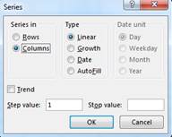
You will need to
scroll to the bottom of the file to figure out what Stop value to enter.
At
this point, you are done with RStudio
Back
in Arc…….
Back in Arc, right-click on your shapefile and Open the Attribute Table again. For
each image segment in the attribute table, we now want to add the spectral
class ID number that we just generated in R using the K-Means unsupervised classification
routine.
In the attribute table window, click on the ![]() Table option button
and go to Joins and Relates-Join. In
the Join Data
dialog box,
Table option button
and go to Joins and Relates-Join. In
the Join Data
dialog box,
Item 1: is the field in your current attribute table
that the Join will be based on; select FID
Item 2: is the Excel file that you just created in R.
You will need to click on the folder icon and point to this file and sheet1$ in
this file
Item 3: is the field in this Excel file to base the
join on. This will be the ID number that you inserted into the first column of
this file.
Click OK.
Arc will chug for quite awhile as it complete the
link for all of the 10,000+ image segments. When it finishes, you will see two
more columns added on the right side of your attribute table, “ID” and “x”.Note that you just created a dynamic link between your
Attribute Table and the Excel file. The information from the Excel file is not saved into the Attribute table at this point…..and
this is OK.
Create
a new raster file:
At this point, we want to create a new raster file
with the same cell size as the original starting image (rededge_ndi2_utm.tif)
but with every pixel having the spectral class number that we just added to the
Attribute Table above. To do this, go the ![]() index
and search for Feature to raster. In
this dialog box, enter:
index
and search for Feature to raster. In
this dialog box, enter:
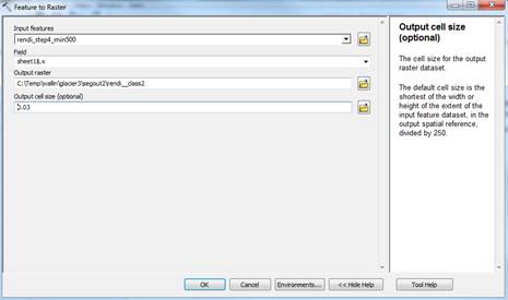
Note that the default Output Cell Size is about 0.44 meters. This is because,
way back when we created the image segmentation, we specified a minimum region
size of 500 cells, which is just under 0.5 meters. So
Arc wants to try to create a raster with a cell size that is about the size of
the smallest image segment. We don’t want this!
We want a cell size of 0.03 m (3 cm) which is the cell size of our original
image. Make sure that you enter this properly. Then hit OK. Arc will
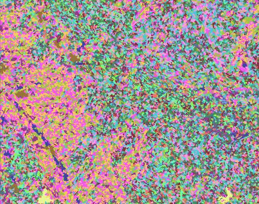
chug for a bit, then add this new raster to your Table of Contents. Take a look at it. Mine looks like this:
a
Export
to ENVI:
Next
we need to move to another software package. Before we do, we need to export
your new raster to a format that ENVI can read. Right-click on your new raster
and go to Data-Export Data. In the Export Raster Data dialog, select a Location and a Name. It is also very important to select a Format which you should set to ENVI. Then Save.
Open
ENVI:
From the Start
button on your computer, go to All
Programs-ENVI-Tools-ENVI5.3 Classic (64-bit). From the ENVI Classic toolbar, go to Open
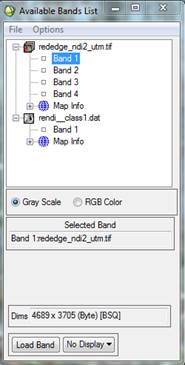
Image File. Open both your spectral class file (mine is called
rendi_class1.dat) and also your original image
(rededge_NDI2_utm.tif). This will bring up your Available Bands List dialog:
Right-click on your class file and go to Edit header. Note that the file type is
currently “ENVI Standard.” Change this to ENVI
Classification. When you do, you will be asked how
many classes are in your file. You have 20.
Entering this value brings up the Class
Color Map Editing dialog. Click OK to
close this. We’ll come back to this shortly. Click OK in the Header Info dialog to close it.
Display
your images:
In the Available
Bands List, go to No Display-New
Display. Click on RGB Color, then,
one at a time, click on Band1, Band2, Band3 in your red edge image, then Load RGB. You should see something like
this:
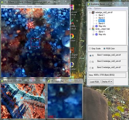
Move the Available
Bands List to the side, go to Display
#1-New Display, then click on Gray Scale, then Band1 in your spectral class image, then Load Band.
You should now see something like this:
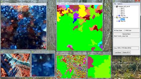
For each display, you have an Image window (upper left), a Scroll
window (lower left) and a Zoom
window (lower right). The red box in the Scroll window is the section displayed
in the Image window. The red box in the Image window is the section displayed in
the Zoom window. You can grab the little red box in either the Scroll or Image
window to change the display.
Link
the displays:
In either Image window, go to Tools-Link-Link Displays. Then OK.
Now, as you move around either display, the other display will move to show
the same location.
Overlay
Classification:
Now the fun begins. We need to assign spectral classes
to information classes. I’m not sure how many
information classes we can break out but at least let’s try for these:
Vegetation
Rocks
Logs
Water
Shadow
To
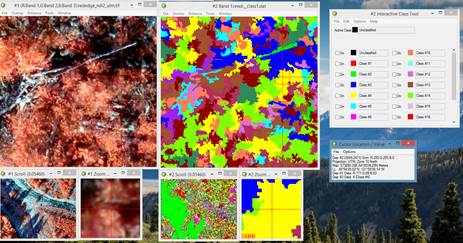
do this, in Image window Display #2 (the one with the spectral classes
displayed) go to Overlay-Classification.
Select our spectral class layer, click
OK. This brings up the Interactive
Class Tool dialog. Also, from the Image window (either one) go to Tools-Cursor Location Value. You should
now have something like this:
I
have moved the scroll window to a forested area in the lower right corner of
the image. Note that my cross-hair is on a yellow blog
that seems to correspond to some vegetation. The Inquire Cursor window
indicates that this is class#4. So, you can go the Interactive Class Tool dialog and go to
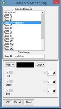
Options-Edit Class Color Names. In
the Class Color Map Editing dialog,
click on Class#4. Under Class Name:
you can then add to the label by calling this something like “vegetation”. Note
that at this point, I’d strongly suggest that you
retain the “Class #4” part of the name. You can also change the color
assigned to this class. For now, change it to black.
Click
OK. Back in the Interactive Class Tool window, you will now see that Class #4 has
your “vegetation” label. You can now click the “ON” box on and off and you will
see a whole bunch of image segments toggle back and forth between the original
color and the new color (black) that you have assigned. What you are seeing is every
image segment in the image that is spectral class#4 turning on and off. As you can see, there are a large
number of image segments in spectral class#4. The same is true for each of the
other spectral classes.
At
this point, you can proceed to assign each of your spectral classes to one
of our five information classes:
Vegetation
Rocks
Logs
Water
Shadow
After
doing so, you will need to save your color scheme and class assignments. You
can do so in the Interactive Class Tool
window by going to File-Save Changes to
file.