Lab VI: Image Segmentation with SPRING

Introduction: In the previous lab exercise, we performed a pixel-based unsupervised classification. This involved the classification of each individual pixel on the basis of spectral data and without taking into account any information about the neighboring pixels. In this lab, we will use a different approach. We perform an image segmentation and unsupervised classification using SPRING v5.2. This software was developed by the Institute for Space Research (INPE) in Brazil. INPE is the Brazilian equivalent of NASA. We have this software loaded on the computers in our lab. You can read a bit more about this software by following this link. If you would like, you can also download it to your own personal computer at home.

As discussed in lecture, image segmentation involves the identification of polygons (regions or image segments) in the image that are made up of pixels that have similar spectral properties. Initially, each pixel in the image is labeled as a distinct region. Each region then grows bidirectionally to include pixels with similar spectral properties. The growth of each region ends when adjacent pixels exceed a pre-defined similarity criterion. Image classification (using an ISODATA algorithm) is then conducted on these regions, rather than on individual pixels. Regions are classified on the basis of the mean spectral properties, the covariance matrix and some spatial properties of the region (e.g. area).

The basic idea of image segmentation has been around for some time. It has not been widely used with Landsat-type data because pixel-based classification works quite well with Landsat-type data. With the relatively recent (initially in 1999 but only widely available within the last 5 years) availability of high resolution multispectral imagery (submeter to 4m such as IKONOS), the use of image segmentation has received renewed interest.

Back to Outline

Objective: In this lab exercise, we will conduct an image segmentation and classification using SPRING. We will then export the resulting spectral/spatial class layer from SPRING and bring it back into ENVI to assign these spectral/spatial classes to information classes and conduct an accuracy assessment. We could conduct this exercise using our familiar Landsat Baker-to-Bay image, but it will be more interesting to use a high resolution image. 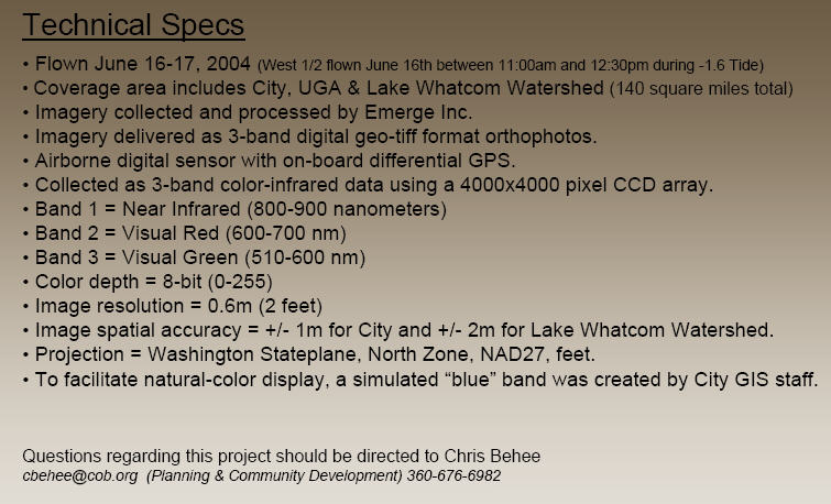We are fortunate to have access to high resolution image that was acquired by the city of Bellingham in June of 2004. The image was acquired using an airborne scanner. The original image has a spatial resolution of 2 feet and it includes three bands.

bham_techspecs

A copy of the original 3-band image in ERDAS Imagine format resides in J:\GEO\GEO_data\BHAM\AirPhoto_Bham\2004_ColorIR\2004_IR_ERDAS This file is huge; it is about 4.6 Gbytes. We will not be using this full image

For the purposes of this lab, I have resampled the original image to a pixel size of 1 meter and reprojected it into UTM with a datum of NAD27. I have also taken a subset of the full study area to create a file of manageable size. The file we will be working with for this lab is:

J:\saldata\Esci442\segwwu\wwu2004cir_1m_utm.img

This file is about 32 Mbytes in size.

Back to Outline

PROCEEDURES

STEP 1: Get yourself a copy of the ENTIRE SUBDIRECTORY J:\saldata\Esci442\segwwu

In my case, my working directory for this lab is C:/temp/wallin13. I have pasted a copy of the entire segwwu subdirectory into this space.

I have done a great deal of the initial work for you, up to and including running the image segmentation for you in SPRING. The reason that I have done this is that getting the image into SPRING and running the segmentation program takes quite a bit of time. Just to let you know how I’ve done all this, you can CLICK HERE to see the full procedures.

Back to Outline

STEP 2: Open your file in SPRING. Start the SPRING-5.2 software (Note that some of the screenshots below are for version 5.1.3 or 5.1.7 but the newer version 5.2 should appear the same).

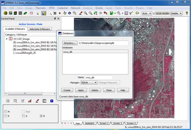
Open the SPRING Database (I have created this for you): We need to begin by opening the SPRING Database that I have created for you. My working folder for this lab is c:/temp/wallin13/segwwu. This includes a folder which I called springdb. This is folder includes the SPRING database that I created for you. As soon as you start SPRING, the Databases dialog box should open (if it doesn’t, go to File-Database from the main SPRING window to open it). In the Databases dialog box, click on Directories and navigate to C:/temp/wallin13/segwwu/springdb (or your working folder) and click OK.

From the Databases dialog box, in the wwu_db will appear in the database Name box and under Manager: SQLiters should appear as the database type. Then click on Apply in the Databases dialog box. The dialog box will disappear.

Back to Outline

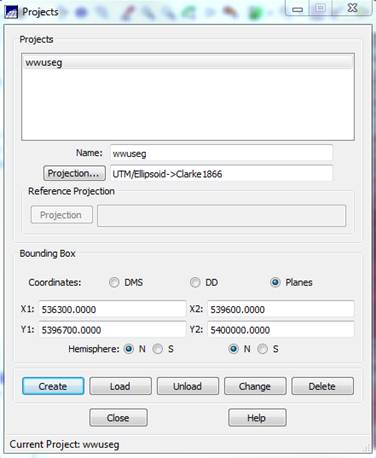
Open the SPRING Project: The SPRING Project defines the projection and bounding box (location and spatial extent) of your image. From the main SPRING toolbar, go to File-Project-Project. In the Projects dialog box, the project name “wwuseg” will appear in the Name box and the coordinates for the bounding box will also appear. Check to make sure that the Northern Hemisphere is specified. After doing so, the project is ready to load so click on the Load button.

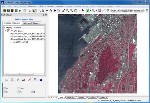
You should then get a screen that looks like this:

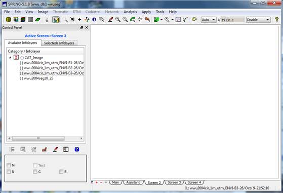
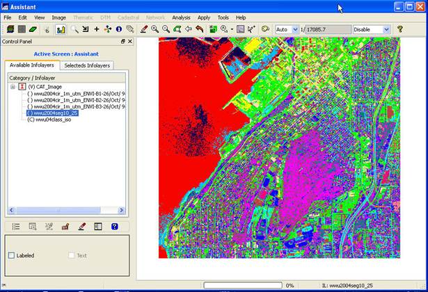
View your image: On the Available Infolayers section of the Control Panel, you will see a list of all the bands in the image, wwu2004…B1, wwu2004..B2, wwu2004…B3 and a layer called wwu2004seg10_25. This is the segmentation.

Let’s start by viewing the image. As in ENVI we display each of our three bands using a unique color gun. Recall that, in our image, Bands 1, 2, and 3 represent the IR, red and green portions of the spectrum, respectively (see the tech specs at the beginning of this lab). To create our now familiar color-IR image, click on Band 1, then click on the R, checkbox in the lower left portion of the control panel. Then click on Band 2 and the G checkbox, then Band 3 and the B checkbox. After doing this, the image should display automatically or you can click on the drawing button to redisplay the image. You should now see something like this:

Back to Outline

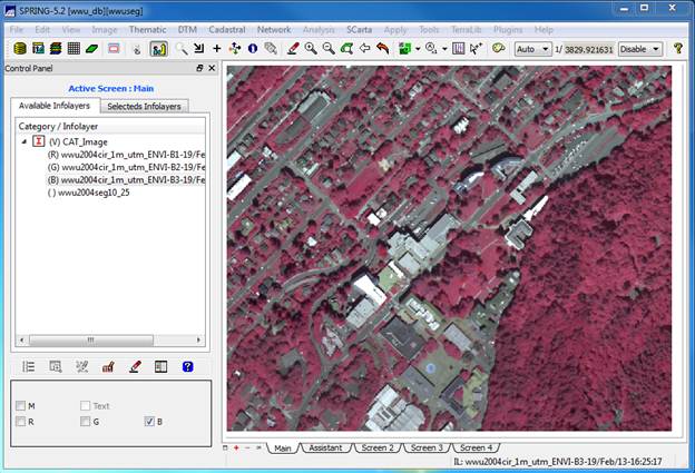
Now click on the Zoom In button a few times to magnify the image.

Back to Outline

View the Image Segmentation: In the Infolayer section of the Control Panel, click on the wwu2004seg10_25 layer to highlight it, then click on the “Labeled” checkbox in the lower section of the Control Panel. This should result in overlaying the segmentation on the image. It will take a moment to load. If it doesn’t do so automatically, then click on the drawing button to display the image with the segmentation overlaid on it.

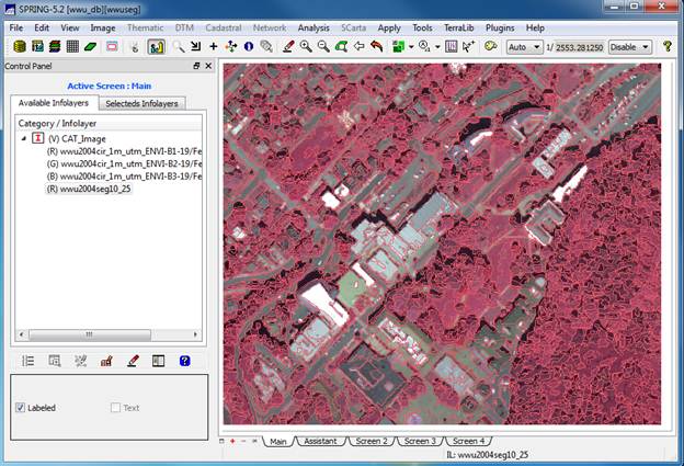
At this point we can see the result of the image segmentation. Note that the individual image segments seem to be fairly homogeneous. This is just what we wanted. Pretty darned cool isn’t it?

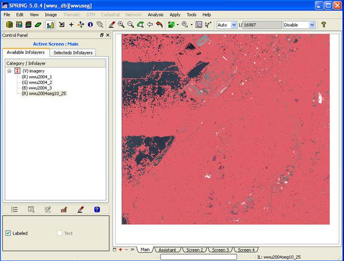
Note that if you try to display the entire image by using the Zoom to Infolayer button , it will take a VERY long time to redraw and you will not be able to see much of anything because the individual image segments are indistinguishable at the scale of the entire image. It will look something like this:

You can spend some time playing with the various zoom functions. On the main SPRING toolbar, click on the zoom cursor button . Move the cursor into the display window, left click on the upper left corner of the area you want to enlarge, then move to the lower right corner and left click a second time. Now go back up to the main SPRING toolbar and click on the enlarge button . Feel free to play around with some of the other zoom tools, including the roaming cursor button (after clicking on this, move your cursor into the display window, then click, drag and release to move around the image at this same zoom level) and the zoom infolayer button (this zooms you back out to the full extent of the image).

Pretty cool isn’t it? If you would like, you can spend some time playing with the zoom functions but don’t spend too much time here. We have lots more to do!

Back to Outline

(Updated to this point by DW 2/19/2013)

STEP 3: Image Classification. We will now perform an ISODATA unsupervised classification of the image. The individual image segments will be classified on the basis of the mean value of each three bands (near-IR, red, green) for all pixels in the image segment, the covariance matrix and the area of the segment.

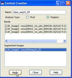
Context Creation: This defines the bands that will be used in the classification and the image segmentation to be used (in the case where you may have run several segmentations based on different similarity and area parameters). From the main SPRING toolbar, go to Image-Classification. In the Classification dialog box, push the Create button. In the Context Creation dialog box, go to the Name: box and enter a name. Something like “class_seg10_25” might be good since we are doing a classification of a segmentation that was created using a similarity value of 10 and a minimum area of 25 pixels. Of course, you could name it something like “Bob”, but that would not be a particularly informative name now, would it? Under Analysis Type: click on the Regions checkbox (note that “regions” are synonymous with “Image segments”). Under Bands click on each of the three bands and under Segmented Images click on our wwu2004seg10_25 segmentation layer. Finally, click on the Apply button.

Back in the Classification dialog box, go to the Contexts box and highlight the context file that we just created (I named mine “class_seg10_25”. You should have only one choice in the Context box.). When you do this, the bands you selected will appear in the Bands box and the name of your segmentation should appear in the Segmented Image box.

Back to Outline

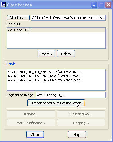
Extraction of attributes of the regions: Now push the Extraction of attributes of the regions button. For each segment (region) in the image, the program will calculate the mean brightness value for each band from every pixel in the segment, it will calculate something called the covariance matrix and it will also calculate the area of each segment. These parameters will be used (below) for the classification. It will take a couple of minutes to complete these calculations (this took about 2 minutes on a computer with a dual-core 3.2 Ghz processors and 4 Gbytes of RAM).

Back to Outline

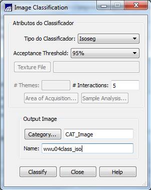
Image Classification: From the Classification dialog box, push the Classification button. In the Image Classification dialog box, go the Classifier box, select Isoseg (this will perform an ISODATA classification) and change the Acceptance Threshold to 95%. Leave the # Interactions: at 5 (OK, I’m not sure what this parameter does? I suspect that this is a typo and they really mean # Iterations, not # Interactions). Leave the Category as a “CAT Image.” Go to the Name box and enter a name for your classification; something like “wwu04class_iso” might be a good choice. In Finally, push the Classify button.

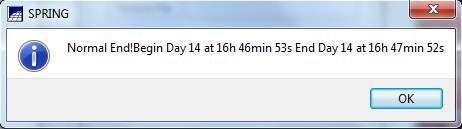
The classification process should be complete in a minute or two. Be patient! You may initially get a “Not Responding message appearing at the top of the Image Classification dialog box. When the classification is complete, you should see something like this. Push OK to close this box and proceed. As soon as you close this box, an Assistant window will appear.

Back to Outline

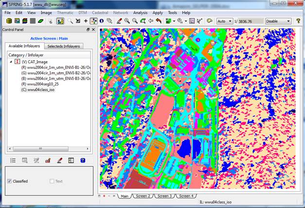
View your classification result (Spectral/Spatial Classes): You will also note that your result (wwu04class_iso in my case) is added to the bottom of the Infolayers list in the Control Panel. It should look something like this.

You can take a look at this, or, minimize the Assistant window, close the Image Classification dialog and go back to the main SPRING display. Go to the Control Panel and scroll down to the bottom of the Infolayers list. You should see your classification result. Click on it to highlight it and click in the Classified checkbox below, then click on the Drawing button . This will show you the same thing that you saw in the Assistant display.

Either way (main SPRING display or the Assistant display), you will now see your spectral/spatial class map. Each region (image segment) will have a solid color and if you look carefully, you will note that some regions have the same color. These represent regions that are in the same spectral/spatial class. The colors in your image may appear a bit different than mine.

Pretty darned cool, isn’t it?

OK, now we need to get this spectral/spatial class map out of SPRING and back into ENVI so that we can assign these spectral/spatial classes to information classes using the same approach we used for the previous lab.

Back to Outline

STEP 4: Export your Spectral/spatial Class layer from SPRING. In the Available Infolayers section of the Control Panel, click on the spectral/spatial class map (mine is called wwu04class_iso) to activate it. Then, on the main SPRING toolbar, go to File-Export-Export Vectoral and Matricial Data.

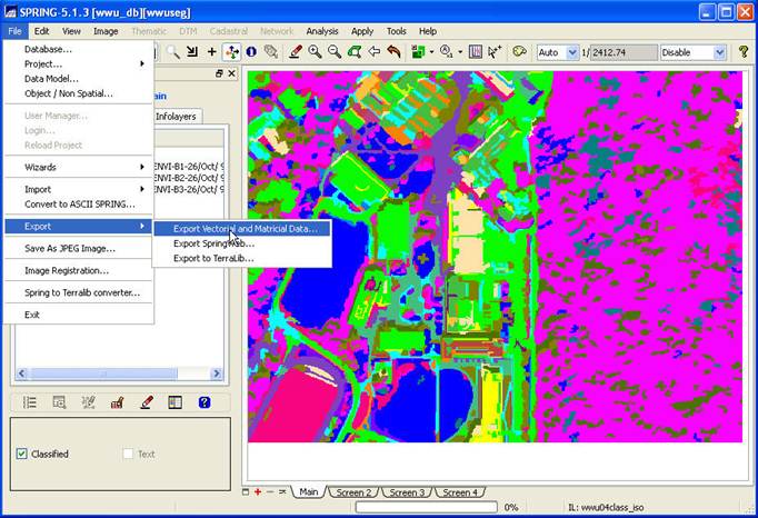
From the Export dialog box, go to the Format: box and select TIFF/GeoTIFF, go to the Infolayer box and click on the spectral/spatial class layer and push the Save button.

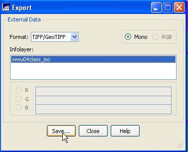
Select a destination folder and output filename. That’s it. We are done with SPRING. From the main SPRING toolbar, go to File-Exit.

Back to Outline

STEP 5: Import your Spectral/spatial Class layer into ENVI.

For some reason, ENVI has a problem reading the TIFF file that is created by SPRING. This TIFF file should be a single band file with the values for this band representing the spectral/spatial class values. ENVI can open the file just fine, but it is opened as a 3-band file with the values for the three bands representing the mix of red, green and blue values that create the same appearance that you saw in SPRING. The spectral/spatial class values are lost. There is probably an easy fix to this in ENVI but I haven’t found it yet. Instead, here is a somewhat convoluted work-around.

Open ArcMap and create a new project. The add the TIFF file to your project by pushing the “add image button and navigating to the folder containing the TIFF file. After doing so (and assuming the check-box is checked) it should look much the same as it did in SPRING (same colors). Right-click on the TIFF file and go to Data-Export Data:

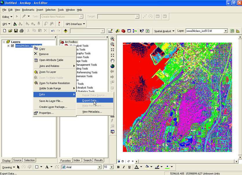
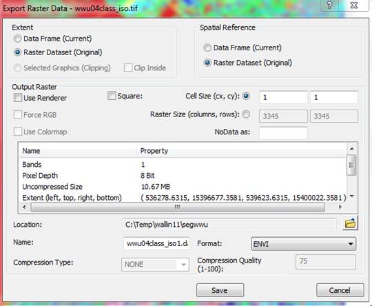
From the Export Raster Data dialog box, specify a Format of ENVI, then select a Location and Name for the output file (I chose to name it wwu04class_iso_ENVI.img) and hit Save.

You can minimize ArcMap but leave it open. We will be coming back to it.

Open your file in ENVI. It should contain a single band. In the Available Bands List dialog, right-click on the image and go to Quick Stats to see how many spectral/spatial classes there are in your image. In my case, there are 36 classes (class #0-35). Right-click on the image again and go to Edit Header. You will note that the image has a File type of “ENVI Standard.” Change this to “ENVI Classification so that we can add a color scheme to the image. When you do this, a dialog box will open asking you to enter the number of classes. After doing so, a Class Color Map Editing dialog box will open. Close this for now; we’ll come back to it. Open this in grey scale in a new display. It should come up with the same colors that you had for this image in SPRING. Now open the original starting file (wwu2004cir_1m_utm.img) and load it into a display as an RGB image with the near-IR, red and green bands loaded into the Red, Green and Blue color guns. We want to link these two displays but, before we can, we need to edit the map info in our spectral/spatial class image.

Editing the Map Info: In the Available Bands List click on the + sign next to the Map Info for both images. You will note that the Map Info for these two files is not the same:

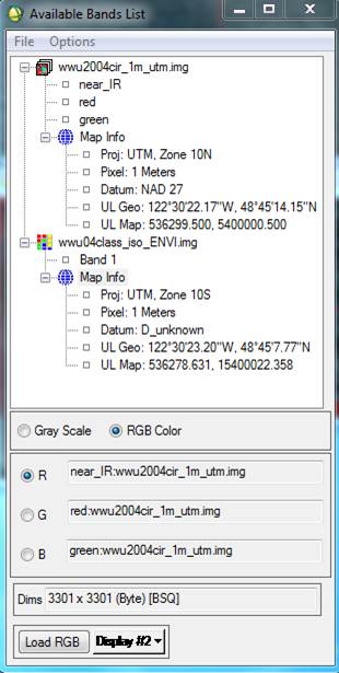
The Map Info for wwu2004cir_1m_utm.img is correct. The Map Info for wwu04class_iso_ENVI.img is not correct. For some reason, some of this information was lost or corrupted somewhere along the line. Among other things, note that the UL Map northing (the second value) is off. Not sure why but, I’ve noted that SPRING has a habit of adding 10 million meters (10,000,000 m = 10,000 km) to the Northing coordinate. We also need to fix the UTM Zone and Datum. So, Right-click on Map Info for your spectral/spatial class image and go to Edit Map Information. Click on Change Projection in the resulting dialog box. In the Projection Selection dialog box, select UTM and Zone “10” (if this is not already set). Change the Datum to “North America 1927.” Also make sure that the Hemisphere is set to “N” NOT “S.” Not sure, but since the software was written in Brazil, maybe it defaults to the southern hemisphere?

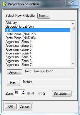
Click OK to close the Projection Selection dialog. Back in the Edit Map Information dialog, take a look at the UTM coordinates. Note that they are now different than the UL coordinates that were showing in the Available Bands List (above). In the case of my image, I got this:

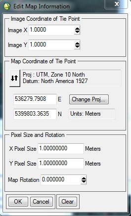
This is a problem. Click on the box containing the Northing coordinate and change to this:

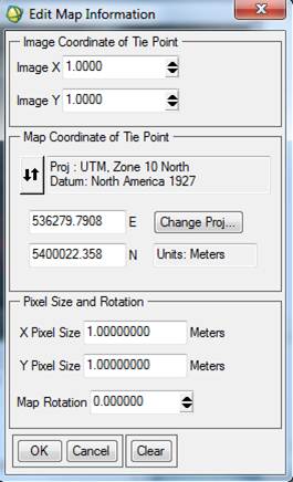
Then click OK to close the Edit Map Information dialog. At this point, the Map Info that is displayed for both images in the Available Bands List dialog should mostly look the same except that the coordinates listed for the upper left corners of the images will be slightly different. I’m not sure why, but SPRING produces an image with a slightly larger spatial extent but the data values for this “extra” area are unclassified. If you look at the header info for both images, you will note that your spectral/spatial class image has 44 more rows and columns than the input image. This means that the upper left corner of your spectral/spatial class image needs to be about 22 m north and 22 m farther west than your input image.

Link you displays: At this point, you should be able to link both displays. Compare the images to see how well they line up. You may need to go back and change the easting (from 536279.791 to 536278.6315) but this probably will not be needed.

Back to Outline

STEP 6: Assign Spectral/spatial Classes to Information Classes. This should be familiar ground for you. In the Image window Menu, you can go to Tools-Cursor Location Value so you can see the spectral/spatial class ID#s for different image segments. From here on, you will follow the same basic approach that you used for the previous lab. Start by using the Crosstabulation approach we used in the previous lab to assign the spectral/spatial classes to information classes. The segwwu folder includes an Excel file with all of the groundtruth data we collected. It is not as large as the dataset we used for the BakerBay image. I’m not sure what to expect, but let’s randomly split the data and use half for the crosstabulation and use the other half later for doing an accuracy assessment.

All of our ground truth files are in J:\saldata\Esci442\segwwu\groundtruth. In addition to your data, we also have data from the past two years so we have about 500 points. The full dataset is in the Excel file lulc3_data.xls. As I did for the previous classification lab, I randomly split the data into training and testing subsets. I then saved separate .txt files for each of the nine LULC codes that we will use (9 training files and 9 testing files). I then pulled these into ENVI to create separate training and testing .roi files (train9class.roi and test9class.roi, respectively). Use the training data to perform a crosstabulation with your spectral/spatial class image. Refer to the Unsupervised classification lab to refresh your memory on the specific instructions on doing this. Use this crosstabulation to guide you in assigning the spectral/spatial classes to these 9 information classes. After doing so, use the Combine Classes function (from the ENVI Main Menu Bar, go to Classification-Post Classification-Combine Classes) to produces a simplified image. Then overlay your test data (test9class.roi) and do an accuracy assessment (again, refer to the Unsupervised Classification lab for specific instructions). You can also try using my ‘accuracy_assessment_template.xls’ to explore the effect of collapsing some of you information classes. Doing so will improve your classification accuracy.

2/23/2010: Important note: Be very careful about DNs vs. Class # in your spectral/spatial class image. I’m not sure why, but in my image, these are not the same. This may or may not be an issue for you. If it is, this leads to huge potential confusion when interpreting your crosstabulation of the the training data and your spectral/spatial class image. For example, in my image the crosstabulation suggests that a DN of 3 seems to correspond to grass. If you open the Cursor Location/Value tool, and put the cursor on any location in the image, you will note that it gives you a separate “Data:” value (this is the DN) and “Class” value. When I place the cursor on a grass practice field on campus, I get this:

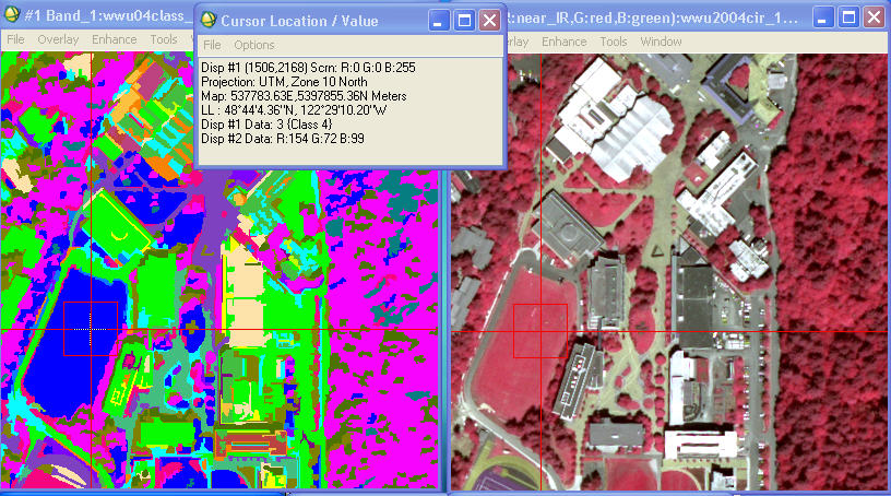
So, this means that when you go to the Class Color Map Editing dialog, you would go to Class 4 (which corresponds to the DN or “Data:” value of 3) to edit the name and color. Sorry, but this is just a quirk of the software.

ArcMap Procedures: As discussed in lab, you can use conditional statements in ArcMap to improve your classification. Start ArcMap and use the button to add your combined classes map that you created in ENVI (mine is called wwu04com_cl.img) and you might also add the original image (wwu2004cir_1m_utm.img). Other layers that you will need are (found in J:\saldata\Esci442\segwwu ):

Bay_mask: This is an Arc Grid that delineates the bay using existing GIS layers. It useful for getting rid of confusion between buildings and water. The bay has a value of zero and the land has a value of “NoData,” however, note that the extent of this grid stops short of the eastern edge of our study area. For this reason, you will need to modify it as described below.

Wwu_sl_el_1m.img:

Veght1mc_n27: This is an Arc Grid that we just recently obtained. It provides LIDAR-derived canopy height (in feet). I found it useful for separating grass, shrubs and deciduous trees. I defined trees as having a height > 6 feet, shrubs were <= 6 feet and >= 2 feet and grass was < 2 feet. Note that, in this layer, all impervious surfaces (including buildings), have a canopy height of 0. More information about this layer (including a version with a larger extent) is available at:

J:\GEO\GEO_data\BHAM\LIDAR_Veg_USGS_2006

This folder includes a readme file with metadata (VegetationHeight2006_Readme.txt). Note this layer was created in the State Plane coordinate system with a grid cell size of 2 feet. Erica reprojected the layer to UTM NAD27 and resampled it to a grid cell size of 1m for our use.

Water: For the water issue, before you can use the Conditional tool with your Bay_mask you’ve got to get the mask to be a full extent and you need to get rid of the NoData value for the land.

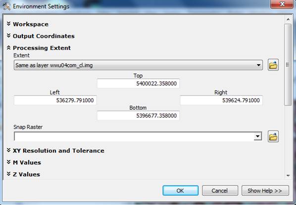
In ArcToolbox, right-click to open the Environment Settings. In this dialog box, go to Processing Extent. Under “Extent” select your combined classes layer that you created in ENVI.

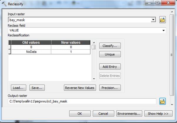
In ArcToobox, go to Spatial Analyst Tools-Reclass-Reclassify, Next Reclassify the Bay_mask to get a mask with a full extent (this works because of the pre-set Environment Extent above). You will need to point to bay_mask as the input raster, specify VALUE as the reclass field, specifiy the old and new values as indicated below and also specify the output raster folder and name. Then click OK:

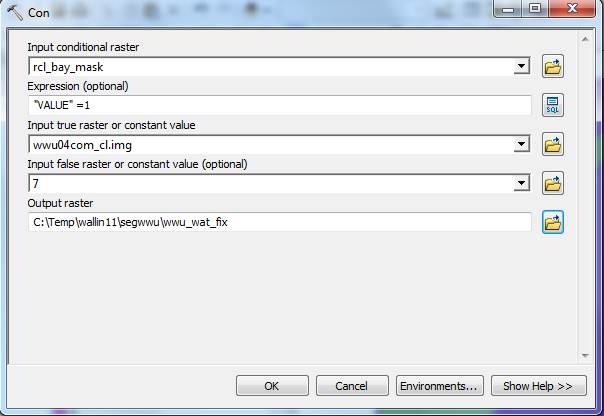
Then go to the Spatial Analyst Tools-Conditional-Con tool to convert all of the water values to 7 and retain the LULC codes for land from wwu04com_cl.img:

To get this to look the same as the original .img file:

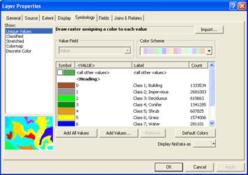
Right-click on the wwu04com_cl.img file and go to the Properties-Symbology tab changed the Show type from Colormap to Unique Values (this didn’t actually change the display, just lets you see/import the actual values for the data layer). Then click on Apply and OK

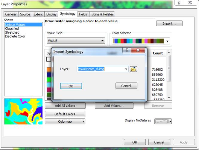
Then right-click on the new wwu_wat_fix GRID and go to Properties-Symbology and use the Import button (upper right) to import the Unique Values symbology from the .img file to the new GRID.

Click on OK in the Import Symbology dialog box, then Apply and OK in the Layer Properties-Symbology dialog and this should bring up the color scheme from wwu04comb_cl.img.

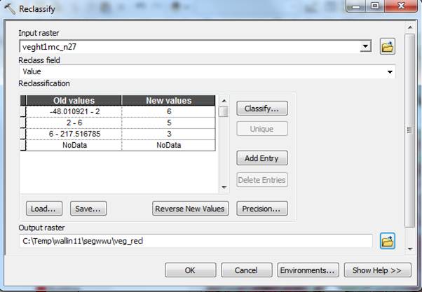
Grass, Shrubs, Deciduous vegetation: We want to do a reclassification that will achieve. For anything in wwu04comb_cl.img that is class 3 (Deciduous), 5 (Shrub) or 6 (Grass):

Anything under 2 feet: should all become 6 (grass)

2 feet – 6 feet: should all become 5 (shrub)

Over 6 feet: should all become 3 (dec)

I’m sure we could write up a single complicated one-step tool that would do all of the conditional statements as a series of if/then statements, but I think it’s easier/faster to break it down into a reclassed veg layer and a simpler Con:

First Reclass the veg layer so it will work in the Con (yes this makes way more grass and shrub than we really want, the bay is grass for example, but it won’t matter in the next step):

Finally, another Con, this time: if the image is 3, 5 or 6 (dec, shrub or grass) use the new values based purely on height, otherwise (values other than 3, 5 or 6) just keep the image values:

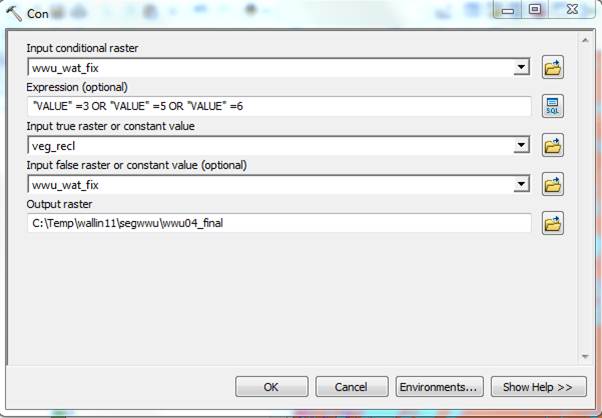
Again, import the symbology from the original .img file to compare the results. Mine looks pretty good. The separation of conifers and deciduous trees on Sehome Hill looks especially good.

At this point, you have an Arc GRID. You can export this to ENVI (right-click on the file, then go to Data-Export data) and do another accuracy assessment and you should see a big improvement for the deciduous, grass and shrubs.

Back to Outline

Return to ESCI 442/542 Lab Page

Return to ESCI 442/542 Syllabus

Return to David Wallin's Home Page