ESCI497Z:
UAS for Environmental Research and Monitoring
Calculating
NDVI for pastures along the North Fork
Objective:
The
objective of this exercise is to process multispectral imagery obtained using a
Parrot Sequoia camera carried by a sUAS to generate vegetation indices for a
pastures along the North Fork of the Nooksack River.
Introduction:
Recall
that the Sequoia has four narrow band 1.2 MP sensors covering the green, red,
red edge and near-IR bands and it also obtains RGB images using a 16 MP sensor.
The narrow band sensors use a global shutter but the RGB sensor uses a rolling
shutter. In this exercise, you will process the images from 4 narrow band
sensors to create a multispectral orthomosaic and further process this to
generate several vegetation indices, including the Normalized Difference
Vegetation Index (NDVI) that we discussed in class. I will also expect you to do
a bit of research on your own to find another vegetation index that can be
calculated using the 4-bands that you will have available to you.
Data:
Go grab the raw images from: J:/Saldata/ESCI-497/N_Fork_Sequoia. Get a copy of
the entire /N_Fork_Sequoia folder. Take a look at the files in this folder. You
will note that it contains TIFF files, that represent each of the four 1.2 MP
multispectral bands and JPG files that represent the 16 MP RGB images. Each
time the shutter is triggered, the camera takes four multispectral images and
one RGB image. The folder also includes one image of the calibration panel that
was taken just before takeoff, in addition to about 150 images that were taken
in flight. The camera was carried by our DJI Matrice 210 quadcopter flying at
120 m AGL. In addition to the raw image files, there is a folder /RGB_ortho,
that contains a tiff file which represents an ortho that I generated for you
from the 16 MP RGB JPG files.
Here is our study area:
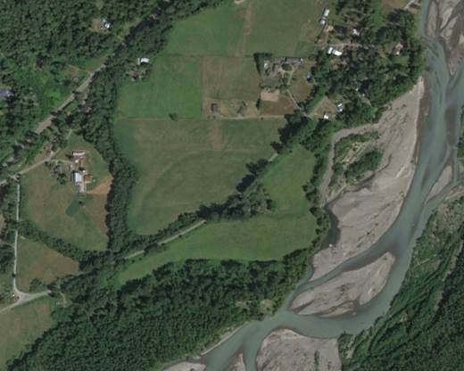
The procedure for loading multispectral imagery is
only slightly different from what you have already done. The process is
described here:
But I will summarize the steps below.
Add
Photos: From the main Agisoft Metashape (AM)
toolbar, go to Workflow-Add Photos as you have done before. You will now see
all the images, both TIFFs and JPG files.
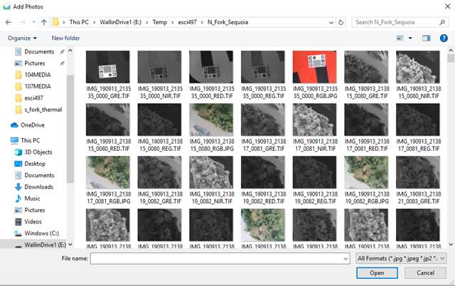
We just want to work with the TIFFs for now so in the
lower right part of the Add Photos dialog, change the file format from All formats to TIFF. When you
do so, all the JPG files will disappear leaving you with just the TIFFs. Like
this:
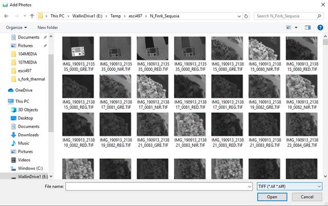
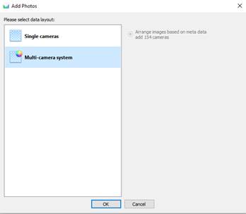
Select all of the files, including the shot of the
calibration panel, then hit “Open.” When you do so, another Add
Photos dialog will appear asking you to select a data layout. You want
to select Multi-camera system. Yes, you are just using a single camera;
the Sequoia. But AM treats each of the four multispectral images as if they
came from separate cameras….which they sort of did. Each band has a dedicated
lens and a dedicated sensor. So select Multi-camera system then hit OK.
In the Photo window, you will just see the images
for the Green band (including the photo of the calibration panel) but the
images for the other 3 bands are there.
Calibrate
Reflectance: From the main AM toolbar, go to Tools-Calibrate
Reflectance. Then hit the Locate Panels button. The software
will scan all the images looking for the photo of the calibration panel. When
it locates it, you will see the following:
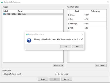
Select “Yes”. It will read the reflectance values for
each band and enter this into the “Panel Calibration” window. It will also try
to read a CSV file and fail in the attempt but all is good. In the parameters
section of the dialog box, select both “Use Reflectance Panels” and “Use Sun
Sensor”. Then click OK.
You can now proceed with the rest of the data
processing as before. Start with Step 5. Here:
HOWEVER,
SEE NOTES BELOW ON SELECTED STEPS!
5.
Align Photos: Go with Medium vs. High accuracy to speed
up processing.
7.
Build Dense Cloud; Set Primary Channel: Try each of the 4
channel but you will probably find that either the Red Edge or the Near-IR
provide the most detail.
Generate both the DEM and the Ortho and take a look at
both by double clicking on them in the Workspace window in AM.
In the DEM, note that there are two old abandoned side
channels of the river that are apparent in the pastures:
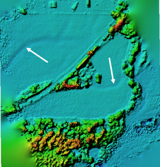
These are a bit lower in elevation and probably have
somewhat finer textured soils and for this reason probably are just a bit
wetter than the surrounding areas of the pasture. What effect do you think this
might have on plant growth? Keep this in mind as we move forward with this
analysis.
10.
Calculate required index information: OK at this point,
you can calculate the NDVI here in AM but I’d like you to move to ENVI (an
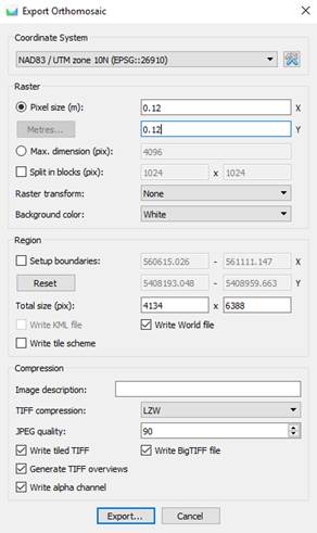
image processing package) to do this……so just go to the main AM toolbar and File-Export-Export
Orthomosaic-Export JPG/TIFF/PNG. I’d suggest you change the coordinate
system to NAD83/UTM zone 10N (EPSG::26910) (you may need to go to “More” to
search for this option) and then change the pixel size to a nice round number.
I chose 0.12 m (12 cm).
Now go to the windows
button ![]() in the lower left of your screen and go to ENVI
5.5-ENVI 5.5 (64 bit). This will bring up the ENVI main window:
in the lower left of your screen and go to ENVI
5.5-ENVI 5.5 (64 bit). This will bring up the ENVI main window:
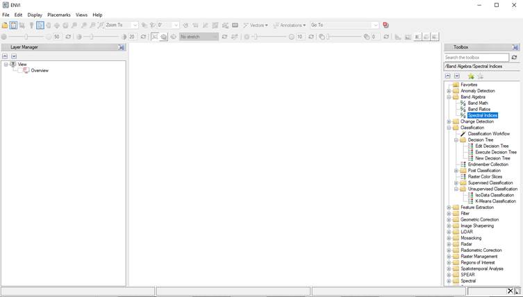
On the main ENVI toolbar,
go to File-Open and navigate to the TIFF that you just exported from
AM. It will probably look something like this:
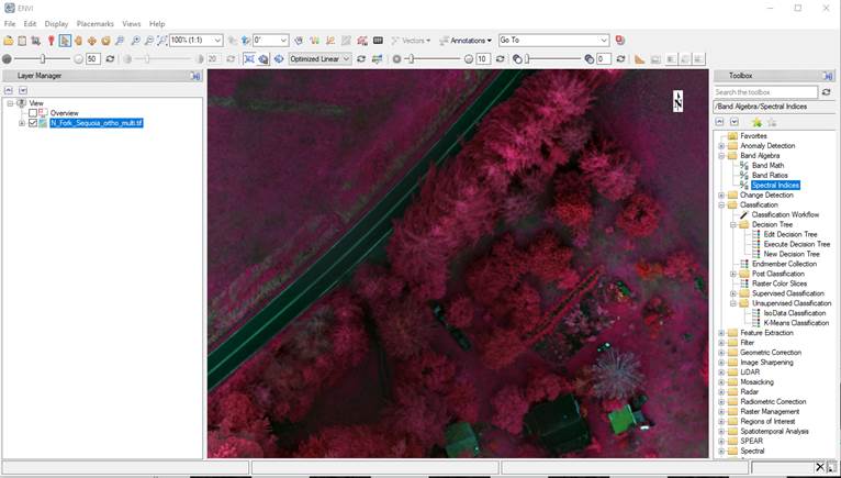
You can use the roller on your mouse to zoom in and
out and click on the little hand ![]() in
the main toolbar and then hold the left mouse button to move around the image.
in
the main toolbar and then hold the left mouse button to move around the image.
Right click on the image name in the Layer Manager and
go to View Metadata. In the View Metadata click on Spectral . Note that there are no
details for the 5 bands. There are really only 4 bands of data in this image.
Band 5 is blank. We want to enter values for the wavelengths for each band. To
do so, click on the Edit Metadata button on the bottom of this dialog box.
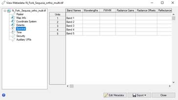
In the Edit ENVI Header dialog box, click
on the Add button ![]() at
the top. In the Add Metadata Items dialog, scroll down and select Wavelength
and Wavelength
Units towards the bottom of the list and then hit OK. Back in the Edit
ENVI Header dialog, scroll down to the bottom to where you see a window
for Wavelength.
You can now click on the Bands one at a time and enter the appropriate
wavelength for each one. You can get this information here:
at
the top. In the Add Metadata Items dialog, scroll down and select Wavelength
and Wavelength
Units towards the bottom of the list and then hit OK. Back in the Edit
ENVI Header dialog, scroll down to the bottom to where you see a window
for Wavelength.
You can now click on the Bands one at a time and enter the appropriate
wavelength for each one. You can get this information here:
https://www.parrot.com/global/parrot-professional/parrot-sequoia
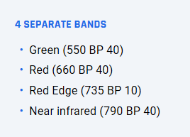
BP just refers to the width of the band. Ignore for
now. The units for wavelength in this case are in nanometers (nm). You can
leave Band 5 at zero since this band is blank. After entering the wavelengths
for the other 4 bands and making sure the Wavelength units is properly set,
click OK
Change
the display: Right click on the image name in the Layer
Manager and go to Change RGB Bands. This enables you to assign any band you want
to the Red, Green and Blue color guns in the display. I’d suggest either going
with 4, 2, 1 for a Near-IR, red, green display or 3, 2, 1 for a Red edge, red,
green display. You can also display each band individually in grey-scale by
putting a single band into all 3 color guns. By doing so, you will note that
the near-IR and red edge bands are the brightest and the red band is the
darkest. You will recall from one of our first lectures that this is because
vegetation is highly reflective in the near-IR and absorbs strongly in the
near-IR part of the spectrum.
Spectral
Indices: We now want to generate a Normalized
Difference Vegetation Index (NDVI) for our image. You will recall, based on
Greg’s video lectures, that this is an index to photosynthetic rate. Recall
that NDVI = (nearIR – red)/(nearIR + red) and this index can take on values
ranging from -1 to +1 but in the real world, the values mostly range from 0 to
1.
Over in the Toolbox window on the right side of
display, go to Band Algebra-Spectral Indices. Clicking on this brings up the Data
Selection dialog. Select your image and click OK. This brings up the Spectral
Indices dialog box which includes a massive number of different
indices. Scoll down to find the Normalized Difference Vegetation Index. Click
on the ![]() button
to select your working folder and give your NDVI image an appropriate name,
then click OK.
button
to select your working folder and give your NDVI image an appropriate name,
then click OK.
Doing so brings up the NDVI in grey scale. We now want
to apply a color scale to this to help us visualize the details in the image.
Color
Ramp: right-click on your NDVI image in the Layer
manager and go to Change color table to select one of the default color ramps.
Selecting Rainbow brings up this:
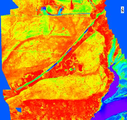
In the second row of the main ENVI toolbar you can
also apply different stretches to this color ramp. The default is “Linear 2%”
but you can play around with the other stretches to see if you find another one
that you prefer.
Raster
Color Slice: You can also right-click on the NDVI image
name in the Layer Manager and go to New Raster Color Slice. This enables
you to assign specific colors to different “slices” of the values in the image.
Here is what the Edit Raster Color Slices dialog looks like:
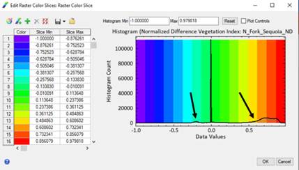
Notice the black line at the bottom of this figure.
This shows the frequency distribution of NDVI values in this image. Note that
there are a few values that are around -0.2, a bunch of values near zero and a
larger bump between ~0.6 and ~0.9. This highest group represents vegetation. You
might choose to slice these values up into perhaps 4-6 “slices” each with their
own color. Here is one (perhaps garish) example:
I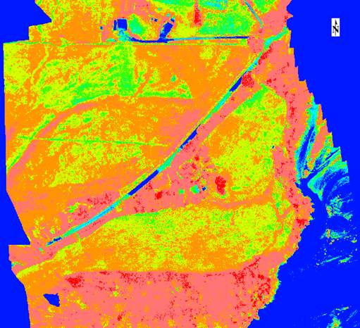
In this version, the shades of blue seem to be things
other than vegetation, including the road, buildings and the open gravel bar in
the river. The other classes appear to be vegetation.. It might be of interest
to see how much of the study area (that is in vegetation) is in each of these
classes. To do so, you can right-click on your raster color slice in the Layer
manager and go to Quick Stats. This brings up the count of the number of pixels
(each 12 cm square in my case) that are in each of the 9 classes that I broke
out. You might have picked more or fewer classes and you probably picked
different class boundaries.
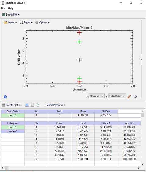
You can go to File-Export to Text file to save
this to a text file that you can then bring into Excel to calculate some
statistics. I’d suggest calculating the % of the vegetation (excluding the
classes you decide ARE NOT vegetation) in each of your NDVI categories.
What
Else? OK, now that you have done this, go back to Toolbox
window on the right side of display in ENVI, go to Band Algebra-Spectral Indices
and explore the other indices that are available. Do a bit of research on the
web for one of these indices. Pick one that can be calculated using the 4 bands
that you have available to you and generate it and play around as you did with
NDVI to help you visualize it.
Lab
report: Prepare a lab report describing your work and your
interpretation of your results. What does the NDVI and the other index that you
selected about these pastures? Which parts of these pastures are growing better
and which are worse and what environmental factors do you feel explain the
variation that is illustrated by your indices?
As always, your lab report is due at the beginning of
lab next week, 11/29 at 1:00PM.
References:
Delegido, J, J. Verrelst, C.M. Meza, J.P. Rivera, L.
Alonso, J. Moreno. 2013. A red-edge spectral index for remote sensing
estimation of green LAI over agroecosystems. European J of Agronomy
46:42-52 Delegido_etal_2013.pdf