407_edgelab

ESCI 407/507: Forest Ecology

Spring 2024

Last updated: 5/3/2024

Lab #5: Comparison of Forest Structure and Composition at Edge and Interior Sites

I. Objective:

The objective of this lab is to compare forest composition and structure at the edge and interior of a stand. We will be visiting is a second-growth stand on lands managed by the Washington State Department of Natural Resources. The adjacent stand was harvested approximately 10-15 years ago. This harvest created an opening in the forest canopy and has altered the microclimate at the edge of the stand we will visit. We should see a number of differences between the edge and interior of this stand. We are particularly interested in differences in size structure, species composition, growth rates, mortality rates, and reproduction of the overstory trees. We will also examine the species composition of the understory. Also of interest is the abundance and structure of coarse woody debris. To gather these data, a number of new sampling techniques will be used. These techniques will also be used in several other lab exercises later this term. Additional sources of information to aid you in the analysis and interpretation of your data will be made available to you. In particular, you should take a look at the paper by Chen et al. (Chen, J., J.F. Franklin and T.A. Spies. 1992. Vegetation responses to edge environments in old-growth Douglas-fir forests. Ecological Applications 2(4): 387-396; Click here to view this article. If this link does not work, go to the WWU Library web page - Online resources - JSTORS and locate the article yourself.).

II. Methodology

Before you begin, remember to record the date, location and brief description of the study area, as well as weather conditions and other factors that may affect your data. Also record the names of everyone in your group and give them credit in your lab write up. You will be working in groups of 3-5. Please rotate positions so you can all have the opportunity to learn the all the methodologies and tools being used.

Your group will need:

1. Two or more 30m tape
2. Four to six DBH tapes
3. Two or three compasses
4. One, 1m² understory quadrat
5. Two or more clinometers
6. One trig. Capable calculator; Bring your own!
7. Two or three rolls of fluorescent marking tape (red or blue best; yellow and green hard to see in the forest)
8. Two laser rangefinders
9. One GPS unit

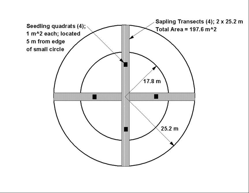
Here is a picture of the circular sampling plot.

Description: Description: Description: Description: Description: 407EDGE

In this lab, you will record information about forest structure and composition in nested circular plots. You will sample two nested plots, one near the edge and the second 150 meters in from the edge of the forest.

A. Setting up the circular sampling plots: All measurements in this lab take place within the bounds of two concentric circles, the inner circle having a projected area of 0.1 ha and the outer circle having a projected area of 0.2 ha (1 ha = 10,000 m²). On level terrain, the smaller inner circle will have a radius of 17.8m and the larger outer circle will have a radius of 25.2m. Just for fun, you should do the calculations yourself to verify that these are correct. Remember that the area of a circle = Pi*r². When laying out these plots on very steep land, some investigators will "correct" the radius of the plot to insure that the projected area of the plot remains constant. This becomes important steep slopes. We will be working on slopes that are fairly steep so we WILL be measuring slope and doing this correction.

To lay out each plot, use your compass and 30m tape to flag eight points, 90 degrees apart at distances of 17.8 and 25.2m from the plot center. Be sure to recover the flagging when you are done collecting data.

B. Measure the Plot Characteristics: Record this information on the “Plot Info” datasheet. Plot characteristics should include:

1: Location: GPS coordinates

2. Site Name/Description

3. Slope: Use your clinometer to measure the slope (in degrees) and record this on the “Plot Info” datasheet. When you enter this data into your Excel worksheet, enter this on the “Slope Correction” worksheet.

4. Date

5. Name and Contact Info for everyone in your group. This is important if there are any questions regarding your data.

C. Measure Canopy Height: Near the plot center, measure the height of the canopy using a tape measure and a clinometer. Record this info on the “Snags” datasheet. The methodology for this will be discussed in the field (and see below). This measurement will be used later to help estimate the height of snags.

D. Tree species counts and diameter measurements: We will measure the diameter at breast height (DBH) for all trees >10cm DBH. Recall that breast height is defined as 1.37m above the ground on the up-hill side of the tree. And gee, WHY do we measure tree diameter at “breast height” and why is this defined as 4.5 feet (137 cm) above the ground on the uphill side of the tree? Why do US Foresters Measure DBH at 4.5 feet?

For small trees (10-50cm DBH), record the species and 10 cm "diameter class" for each tree (10-20cm, 20-30, 30-40, 40-50; See data sheet) that is within 17.8 m of the plot center (small circle only). We do not need to record the exact diameter for these trees, only the diameter class.
For large trees (>50cm DBH), record the exact DBH measurement for all trees that are within 25.2 m of the plot center (large circle). This means that all large trees (>50cm DBH) in both the small and large circle get counted. Small trees (10-50cm DBH) get counted only if they are in the small circle. Large trees (>50cm) are less abundant than small trees so we need to sample a larger area to get an accurate estimate of their density.

E. Sapling counts by species: Use a compass and a 30m tape to create four 2 meter wide belt transects. The transects begin at the plot center and run out to the edge of the 0.2 ha plot at 0, 90, 180 and 270 degrees. Use your arms to estimate the 2 m width and record the number and species of all trees less than 10 cm DBH and greater than breast height with that strip. The total area sampled by these transects is [(2*50.4)+(2*48.4)] = 197.6 m² .

F. Groundcover estimates: We will be using four quadrats, each 1 m². In each quadrat, estimate coverage to the nearest 5%. Record all shrubs and ferns by species, but lump all herbaceous and all grass species into two composite classes. Use your compass to place the quadrats due north, south, east and west, five meters in from the edge of the 0.1 ha circle as shown in the figure above. Record your percentages in the table provided. For each quadrat, your percentages (including bare ground) must add up to 100%. You should also record the number of tree seedlings, by species, in each quadrat.

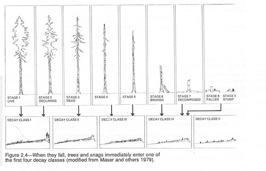
G. Snags: Measure the DBH and estimate the decay stage (see accompanying figure and table) of all standing dead trees (snags) within the 0.2 ha plot. Typically, snags are only recorded if they are at least 1.37 m tall (“breast height”), HOWEVER, see the Stump section below. Record this information in the table provided. Also, estimate the height of each snag as a percentage of the overall canopy height. If the snag is rather short (ex. 3-5m) it may be easier to simply estimate the height in meters. Note the condition of the top of the snag. Is it broken off or mostly intact (tree comes to a point)? This information will be used in an upcoming carbon budget lab.

Stumps: This second-growth stand was logged for the first time in about 1920. Throughout the stand, there are numerous rotted stumps left over from this era. Collecting information about these stumps will allow us to reconstruct a few characteristics of the pre-harvest old-growth stand. All stumps, even those that are heavily rotted and are less than breast height, should be recorded. The heavily rotted stumps that obviously date from the 1920s-era harvest should be recorded as stage 9. This will distinguish them from the other snags that are the product of natural mortality of trees that have regenerated since the 1920s harvest. Be sure to record the height of all snags and stumps. Note that in many cases, the old springboard notches can still be seen in these old stumps.

Physical characteristics of Douglas-fir snags by deterioration stage, western Oregon (adapted from Table 2.3 in Maser et al. 1988)

	Decay Stage
Snag Characteristic:	I	II	III	IV	V
Limb & branches	All present	Few limbs, no fine branches	Only limb stubs	Few or no stubs	None
Top	Pointed	Broken	Broken	Broken	Broken
Bark remaining (%)	100	Varies	Varies	Varies	<20
Sapwood presence	Intact	Sloughs	Sloughs	Sloughs	Gone
Sapwood condition	Sound, incipient decay, hard, original color	Advanced decay, fibrous, firm to soft, light brown	Fibrous, soft, light to reddish brown	Cubical, soft, reddish to dark brown
Heartwood condition	Sound, hard, original color	Sound at base, incipient decay in outer edge of upper stem, hard, light to reddish brown	Incipient decay at base, advance decay throughout upper stem, fibrous, hard to firm, reddish brown	Advanced decay at base, sloughing from upper stem, fibrous, or cubical soft, dark reddish brown	Sloughing, cubical, soft, dark brown or fibrous, very soft, dark reddish brown, encased in hardened shell
Estimated age at which snags reach a given stage of deterioration:
4-18 inches DBH	0 – 4 yrs	5 – 8 yrs	9 – 17 yrs	>17 yrs	Fallen
8-19 inches DBH	0 – 5 yrs	6 – 13 yrs	14 – 29 yrs	30 – 60 yrs	>60 yrs
>19 inches DBH	0 – 6 yrs	7 – 18 yrs	19 – 50 yrs	51 –125 yrs	>125 yrs

Description: Description: Description: Description: Description: decay_cl (Fig 2.4 from Maser et al. 1988)

H. Coarse Woody Debris (CWD): For all fallen trees within a 0.05 ha plot (1/4 of our big circle; I’ll randomly select which ¼ to use), measure the length and the diameter of the small and large ends. Do this for all pieces with a minimum diameter of 10 cm at the large end. Measurements should only be taken for those sections that are within the 0.05 ha plot. For pieces that do extend beyond the edge of the plot, take diameters of the piece at the plot edge. You should also record the decay class for each piece using the accompanying table below. It is OK to estimate the diameter if the decay class does not permit accurate measurement.

A 5-class system of decay based on fallen Douglas-fir trees (Adapted from Table 2.6 in Maser et al. 1988)

Decay Class	I	II	III	IV	V
Bark	Intact	Intact	Trace	Absent	Absent
Twigs (3 cm)	Present	Absent	Absent	Absent	Absent
Texture	Intact	Intact to partly soft	Hard, large pieces	Small, soft blocky pieces	Soft and powdery
Shape	Round	Round	Round	Round to oval	Oval
Color of wood	Original color	Original color	Original color to faded	Light brown to reddish brown	Red brown to dark brown
Portion of tree on ground	Tree elevated on support points	Tree elevated on support points but sagging slightly	Tree sagging near ground	All of tree on ground	All of tree on ground
Invading roots	None	None	In sapwood	In heartwood	In heartwood

When we get to the analysis phase of this lab, you will need to calculate the volume of each piece of coarse woody debris. To do this, we will assume that the volume of each log can be calculated as the frustrum of a cone. This is simply a cone with the top cut off. Just in case you don’t happen to remember the formula for the frustrum of a cone, here it is:

Volume = L [ BA_top + BA_bottom + sqrt (BA_top*BA_bottom)]/3

Where: L = length of the log
BA_top = Basal area of the top of the log
BA_bottom = Basal area of the bottom of the log
sqrt( ) = the square root of the quantity in ( )

Basal area is simply the cross-sectional area of the log at a given point. This is calculated using the familiar formula for the area of a circle:

Area = Pi (r)²

In our case, since we measured the diameter of the log (or tree) rather than the radius:

Basal area = Pi (diameter/2)²

Where: Pi = 3.1416

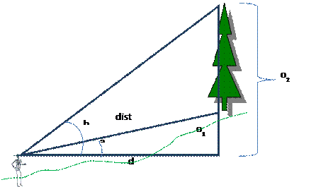
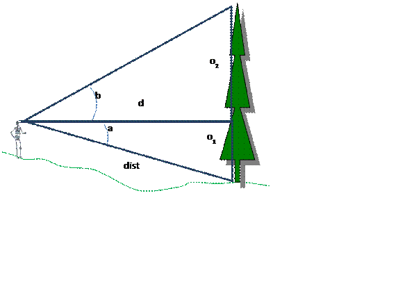
Tree Height Calculation: Just in case you need a refresher on your middle school trigonometry, here is how you calculate tree height. In the field, you will measure canopy height by selecting a representative tree. You then back away from the tree some distance and use a clinometer measure the angle, in degrees, to the top of the tree and the angle to the bottom of the tree. Record these angles and the distance to the base of the tree (measured with a tape measure). You will need to be at least 30 meters from the base of the tree; perhaps more than this. Canopy height is then calculated as follows:

a: angle (in degrees) to base of tree
b: angle (in degrees) to top of tree
"Uphill" angles (like a and b in lower figure) are entered as a positive value and
"downhill" angles (like a in upper figure) are entered as negative value.
dist: distance (m) along slope to base of tree
d: horizontal distance (m) from observer to trunk of tree
o1: "opposite" side for angle a (m)
o2: "opposite" side for angle b (m)


o1 = sin(a)*dist
d = cos(a)*dist
o2 = tan(b)*d

total tree height = o2 - o1 = (tan(b) * (cos(a)dist)) - (sin(a)dist)
This equation will work even if either the angle downslope or upslope is zero.
NOTE: trig functions in Excel expect angles in radians not degrees
To convert angles in degrees to angles in radians: radians = degrees * PI()/180


Trig function review: http://www.grc.nasa.gov/WWW/K-12/airplane/sincos.html

III. Data Analysis:

Your team will compile your data using the format on the data sheets that I provide. These data sheets are printouts of worksheets from this Excel workbook.

forest_data_anal_template.xls

When you get home, you will need to transfer the data from your paper data sheets into the appropriate worksheets in this Excel file. Note that this Excel file is set up to do a large number of calculations for you. It is essential that you fill in the data on each of the “Raw….” Worksheets:

Raw Tree Data

Raw Understory/Sapling

Raw CWD

Raw Snags

Also be sure to fill in the Plot Info worksheet! All of the other worksheets are linked to these “Raw…” pages. Using this excel file will save you many dozens of hours. If you fill in the raw data correctly, these linked worksheets will carry out most of the calculations for you. This will include converting your raw stem counts into stems per hectare and calculating basal area per hectare. Take careful look at these pages and follow the links to figure out how these calculations are done.

For each plot, I want to receive a single Excel file containing ALL of the data. Don’t have one person send me the tree data, another the snag data, etc. I don’t want to try to figure out how to piece the data together (Gee, does this tree data go with this snag data or this other snag dataset?). Save your file using a unique name; something like “smith_tues_edge_2023.xls.”

Please email your complete data sets directly to me no later than NOON on the day after your lab. I will post all of these class data on Thursday (for the Wednesday lab) or Saturday (for the Friday lab). The sooner you send them the sooner I can post them. Note that your lab report will be based on using data from BOTH the Wednesday and Friday labs.

NOTE: All datasets must be received by me in complete form by NOON on the day following your lab. Failure to turn your data in on time will result in a penalty of one full letter grade on your lab report for EVERYONE in your group. There are no exceptions and no excuses. I don’t care whose “fault” it is. It is the collective responsibility of each member of each group to see to it that this gets done. This is a simple task. See to it that it gets done!

In addition to the data we collect, we will also be using data collected in this same stand in previous years. We will all be working with the same data. These data present a very large number of potential comparisons. Take a look at the paper by Chen et al. (1992. Ecological Applications 2:387-396) that is available on the web (see link to this above). This paper will provide some background and a starting point for your analysis. To make your lives simpler, you can limit yourselves to the analyses suggested below. More creative analyses will be rewarded!

Click on each file below to open each excel file. Save a copy of each of these files. These files contain the data from past years and instructions on where your data should be pasted in. These files will serve as templates to use for completing your analysis. Links in these files will make it easier for you to do most of the calculations. Be careful only to make changes in the field that I have indicated. If you mess up any of the links/formula, simply start over with a new copy of the file. (Note: When opening these files, if you get a message asking if you want to update links to other files, click NO).

The spreadsheets will save you an enormous amount of time in preparing the tables and figures below. I will spend time in class on Friday, 5/5 explaining how to use these spreadsheets. I will not be posting instructions on the use of these spreadsheets on the web page. If you miss class, check with a classmate or make an appointment to see me or either of the TAs. Please do not wait until the last minute to begin working on your lab report!

Table 1: Mean and standard deviation (among plots) of tree density (stems/ha) by species and for all species. Also include separate values for all conifers and for all hardwoods. This is for trees >10cm DBH only. Calculate separate values for the edge and interior plots. Compare these means using a two-sample t-test or single factor ANOVA in Excel, Statistix, SPSS or some other software package.

Table 2: Mean and standard deviation (among plots) of basal area (m²/ha) by species and for all species. Also include separate values for all conifers and for all hardwoods. This is for trees >10cm DBH only. Calculate separate values for the edge and interior plots. Compare these means using a two-sample t-test or single factor ANOVA in Excel, Statistix, SPSS or some other software package.

Figure 1: A histogram showing the tree size class distribution. Calculate the mean stem density (stems/ha) for each size class. You should include a pair of bars for each size class (seedlings, saplings, 10-20, 20-30, 30-40, 40-50, 50-75, 75-100, 100-150...). You may choose some other size class intervals for the trees over 50cm if you wish. One bar in each pair presents mean values for the interior plots and the other presents the mean values for the edge plots. If you want to get fancy, you can try to include the 95% confidence interval for each of these mean values. For this figure, we lump all tree species together.

Table 3: Understory composition. Mean and standard deviation (among plots) of Total percent cover and percent cover for all shrub species and for the herbaceous and grass classes. Calculate separate values for the edge and interior plots. Compare these means using a two-sample t-test or single factor ANOVA in Excel, Statistix, SPSS or some other software package.

Table 4: Snags. Mean and standard deviation (among plots) of snag density (stems/ha) and snag basal area (m²/ha). Coarse Woody Debris (CWD) Volume (m³/ha). Calculate separate values for the edge and interior plots. Compare these means using a two-sample t-test or single factor ANOVA in Excel, Statistix, SPSS or some other software package.

Figure1.xls Updated for 2024 You should add note to ALL figure/table legends RE the number of plots used in the analysis
Table1.xls   Updated for 2024
Table2.xls   Updated for 2024
Table3.xls   Updated for 2024
Table4.xls   Updated for 2024

Links to 2024 data will be posted below

int_wed2024.xlsx All data look OK

Edge_Wed2024.xlsx All data look OK

Unfortunate mix up for the Friday lab! On Wednesday, we were told that we could leave all of our field gear in one of the vans and that we’d have this same van on Friday. However, when we picked up vans today, we were given different vans and the van with all of our field gear left earlier today for a different class. Sooooo, no field gear meant that we could not collect any data. Soooo, here are files for an edge and interior plot that we collected last year.

Int_mon_2023.xlsx Posted! 5/2 9:30AM Data looks great!

Edge_Mon_2023.xlsx Posted! 5/2 9:30AM Data looks great!

This gives you data for 4 plots (2 edge and 2 interior) that you can use for your lab reports along with other data from previous years that are in the Table1-4 and Figure 1 excel files.

wed_edge2016.xls (looks OK)

tues_edge2016.xls (looks OK)

Monday_int2012l.xls

Monday_edge_2012.xls

Tues_Int_2012.xls

Tues Edge 2012.xls

IV. Due Date for Lab Reports: Lab reports are due by 9:00 AM on Wednesday, May 8. As on all lab reports, there is a 5% per day penalty for turning in your report late. Be sure to check the Lab Index page for information on the proper format, organization and grading criteria for your lab reports.

V. Literature Cited on this web page (both papers are available online):

Chen, J., J.F. Franklin and T.A. Spies. 1992. Vegetation responses to edge environments in old-growth Douglas-fir forests. Ecological Applications 2(4): 387-396

Maser, C., R.F. Tarrant, J.M. Trappe, and J.F. Franklin. 1988. From the forest to the sea: a story of fallen trees. PNW Research Station, USDA Forest Service; General Technical Report PNW-GTR-229, Portland, Oregon, 153 pages (Caution! This is a very long publication! Please do not print out a copy of this one!)

(Click here to view the online bibliography for links to these two papers)

Return to ESCI 407/507 Lab Index Page

Return to ESCI 407/507 Syllabus

Return to David Wallin's Home Page